How Training Works — The training loop

The page before this one, backpropagation, finished with a tiny network, a loss of 0.7396, nine gradients and one step that brought the loss down to 0.1929. That was one step on one example. A real training run is that same step repeated hundreds of thousands of times over a whole dataset, inside a loop. The loop also has to decide how big each step should be, when to make the steps smaller, what the weights held before the first step, and what to save so that a run which stops can be started again.

This page is about that loop. It writes the loop out in the order a computer runs it and explains each line. It then replaces the simple step of the page before with the rule that almost everyone actually uses, which keeps a running average of the gradients instead of trusting the newest one. After that it covers three decisions that are made around the loop rather than inside it. Those three are how the learning rate changes as the run goes along, what the weights are set to before the first step, and how you read the curve that the run produces.

This page is for a reader who has read the three pages before it in this chapter. It assumes the loss from the score of being wrong, and the gradient, the learning rate, the mini-batch and the epoch from gradient descent, and the forward and backward passes from backpropagation. The maths stays at multiplying, adding and keeping a running average. A running average is an average of the recent values of something, weighted so that the newest values count most.

Every number on this page comes from a real run of a small network written in NumPy on simulated data, and the script that drew the pictures prints each one. By the end you will be able to read a training loop line by line, choose an optimiser and a schedule and say why, and look at a loss curve and name what is wrong with the run.

Contents#

The loop, in the order the code runs
Momentum, which is a running average of the gradient
Adam, and why AdamW keeps the shrinking separate
Learning-rate schedules and warmup
Where the weights start
Reading the curve, the time a run takes, and the checkpoint
Where to read next
Using it in Python

1. The loop, in the order the code runs#

Everything that the three pages before this one explained happens inside seven lines of code. Those seven lines run in the same order every time, so the first thing to do is to write them down.

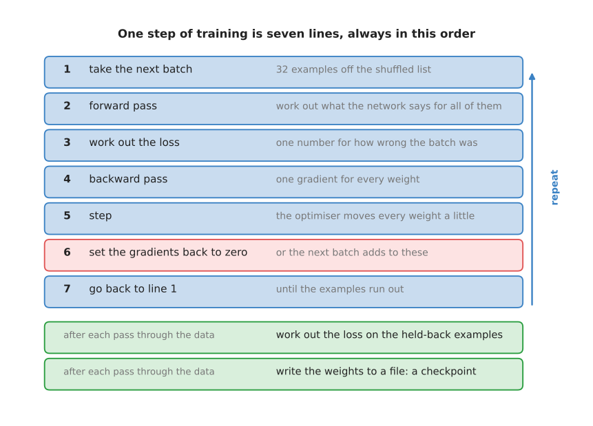
A list of seven numbered boxes for the seven lines of the loop, with the zeroing line marked in red and a repeat arrow up the side, and two green boxes underneath for the end of a pass

The seven lines are: take the next batch, forward pass, loss, backward pass, step, set the gradients back to zero, and go back to line 1; and two more things are done at the end of each pass through the data.

Line 1 takes the next batch. A batch is a small group of examples drawn from the training set in a shuffled order, as explained in gradient descent. Line 2 is the forward pass, which calculates what the network says for every example in that batch at once. Line 3 averages those examples' losses into one number. Line 4 is the backward pass, which gives one gradient for every weight.

Line 5 is the step. The thing that takes the step is called the optimiser, which is the rule that turns gradients into changes to the weights. On the page before, the optimiser was the simplest one there is, which subtracts the learning rate multiplied by the gradient. The next two sections replace it with something better.

Line 6 sets every gradient back to zero. This line exists because frameworks add each backward pass into the gradient that is already stored, rather than replacing it. That behaviour is useful when you want to join several small batches into one large one. However, it is a disaster when you forget it, and the two pictures below show what forgetting it does.

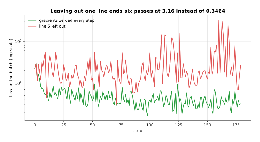
Two loss curves over 180 steps on a log scale, one from a run that zeroes the gradients and one from a run that does not

With the gradients zeroed every step, the loss after six passes through the data is 0.3464; with line 6 left out it is 3.16, nine times worse.

The cause is visible in the gradient itself, because the number the step uses grows every time a new backward pass is added into it.

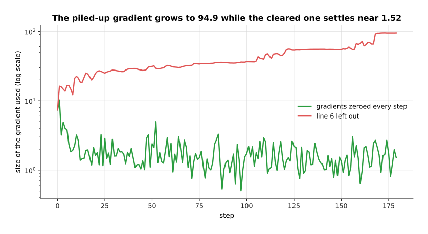
Two lines of gradient size over 180 steps on a log scale, one climbing steadily and one staying flat

The gradient being used grows from 7.361 to 94.9 when it is never cleared, while the cleared one settles near 1.52.

Line 7 goes back to the start. The loop runs until the training set is used up, and one pass through the whole training set is called an epoch. The counting is worth doing once by hand, because the number of steps in a run is the only thing that decides how long the run takes.

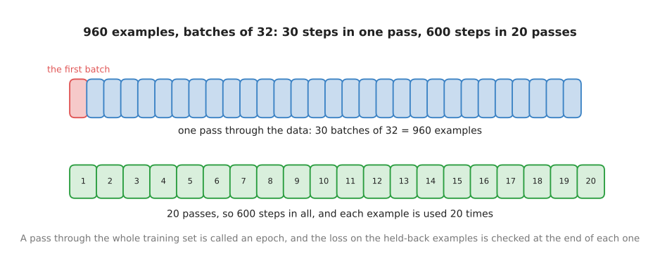
A row of 30 small boxes for the batches in one pass and a row of 20 boxes for the passes, with the counts written underneath

A training set of 960 examples in batches of 32 gives 30 steps in one pass through the data, so 20 passes are 600 steps, and the network is shown 19,200 examples in all, which is each of the 960 exactly 20 times.

At the end of each pass two more things happen, and both of them are drawn in green in the first picture. The loss is calculated on a set of examples that the loop never trains on, which is called the held-back set, and the weights are written to a file. The next chapter explains the held-back set properly in overfitting and generalisation, and section 6 of this page explains the file.

One warning about the loss you see go past on the screen. The loss on line 3 is the loss of one batch of 32 examples, and not the loss of the training set. So it jumps up and down from step to step even when the run is going perfectly.

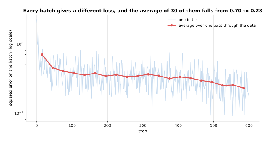
A chart of the loss on every one of 600 steps in pale blue with the average over each pass drawn through it in red

In the first pass the batch losses run from 2.242 at the highest down to 0.349 at the lowest, while the average over the 30 batches of a pass falls steadily from 0.699 to 0.229.

The jumping comes from the batch, because 32 examples drawn at random are sometimes easier than average and sometimes harder. So the average over a whole pass is the number worth watching. That is why training curves are almost always drawn with one point per pass rather than one point per step.

2. Momentum, which is a running average of the gradient#

Line 5 of that loop was the simplest possible optimiser, and this section replaces it, because the simple rule wastes most of its steps on a problem that every real network has. The problem is that the loss is far steeper in some directions than in others.

The picture below uses a loss with only two weights, so that the whole thing can be drawn on paper. The loss cares about one of those two weights a thousand times more than about the other. A map drawn with lines joining the points of equal loss is called a contour map, and on such a map a long narrow valley means exactly that difference in steepness.

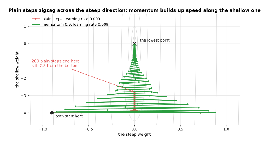
A contour map of a long narrow valley with two paths drawn on it from the same starting point, one in red that barely moves and one in green that zigzags along the valley

Both runs use the same learning rate of 0.009, and after 200 steps the plain rule has crawled from -4.0 to -2.7948 along the valley while momentum has reached -0.0560.

The plain rule is stuck because one learning rate has to serve both directions. It must be small enough that the steep direction does not overshoot, which means jump past the bottom and come out higher on the other side. Once the rate is that small, it moves the shallow direction almost not at all. So the run spends its time crossing the valley instead of going down it.

The rate of 0.009 is not an arbitrary choice. It is the largest round number that this plain rule survives on this loss, and just above it the run is destroyed.

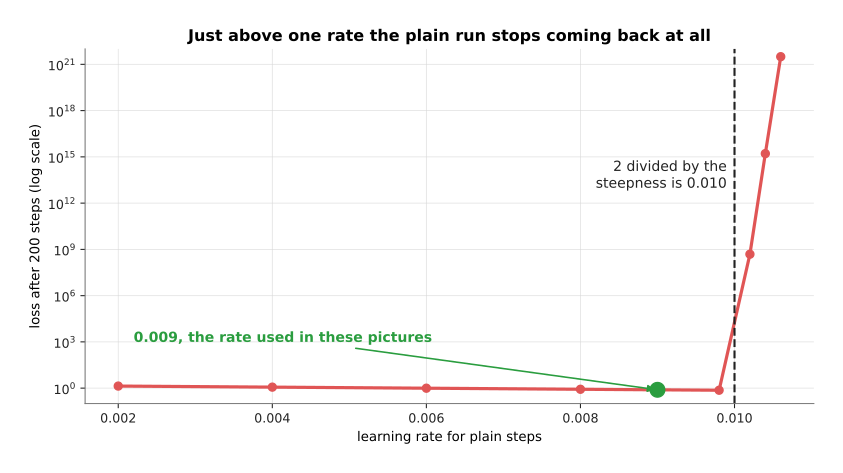
A line of loss after 200 steps against learning rate on a log scale, flat up to 0.0098 and then rising almost vertically

Every rate up to 0.0098 leaves the loss between 0.73 and 1.36, and a rate of 0.0102 leaves it at 4.9e+08, because the rate at which plain steps stop coming back is 2 divided by the steepness, which is 0.010 here.

Momentum fixes the slowness by keeping a running average of the gradients instead of using only the newest one. The rule has two lines. First, the average is set to 0.9 multiplied by the old average, plus the new gradient. Second, the weights move by the learning rate multiplied by that average. The number 0.9 is the only setting, and it says how much of the past is kept.

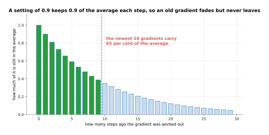
A bar chart of how much of each past gradient is still in the running average, falling from 1 to 0.047 over thirty steps

With 0.9 kept each step, the gradient from 30 steps ago still counts 0.047 against 1 for the newest one, the shares of all the past gradients add up to 10.0, and the newest 10 gradients carry 65 per cent of that.

Keeping the past is useful because of what it does in the two directions. In the steep direction the gradient changes sign at every step, because the run keeps crossing the valley.

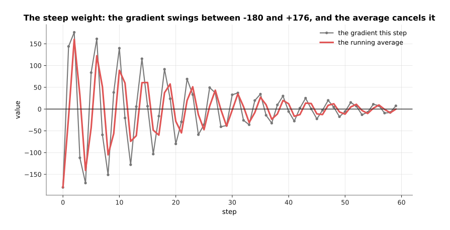
A chart of the gradient and its running average over sixty steps for the steep weight, with the gradient swinging between large positive and large negative values

In the steep direction the gradient swings between -180 and +176, so the positive and negative values land on top of each other in the average and cancel, and the average never grows beyond the size of a single gradient.

In the shallow direction the gradient keeps the same sign at every step, because the run is always on the same side of the bottom.

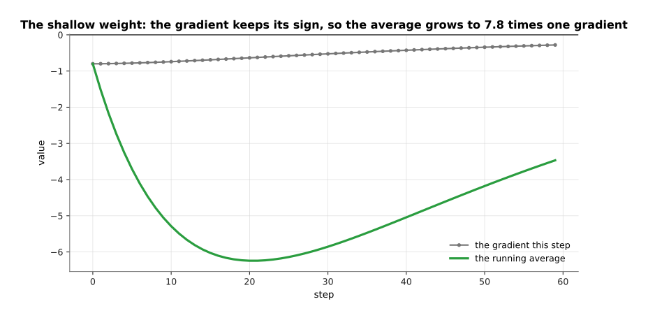
A chart of the gradient and its running average over sixty steps for the shallow weight, with the average growing far beyond the gradient

In the shallow direction the gradient stays near -0.80 every step, so the average grows to -6.24, which is 7.8 times one gradient.

That is the whole trick, in two pictures. Where the gradient keeps pointing the same way, the average grows and the steps get longer, so the run speeds up. Where the gradient flips sign every step, the values cancel in the average, so the steps stay short and the zigzag is damped. The result is a much faster run at the same learning rate.

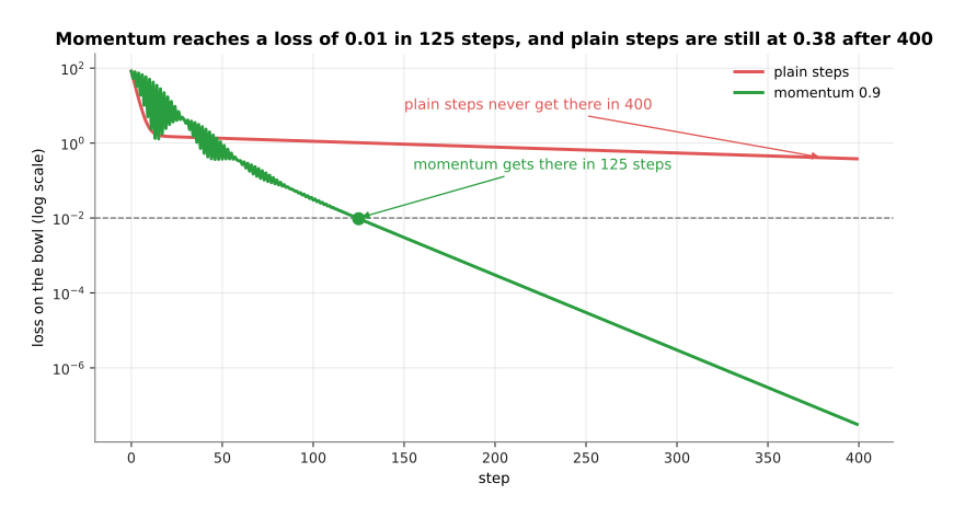
A chart of the loss against step for the two rules on a log scale, with momentum crossing a dashed line at 0.01 after 125 steps

Momentum brings the loss below 0.01 in 125 steps, and the plain rule has still not reached 0.01 after 400 steps, where it sits at 0.380.

Momentum costs one extra number stored for every weight, so it needs as much memory again as the weights themselves. The obvious alternative is to raise the learning rate instead of keeping an average, but the picture of the cliff above shows that the steep direction forbids this. So paying for one more number per weight is the better deal.

3. Adam, and why AdamW keeps the shrinking separate#

Momentum made the steps longer where the gradient was steady. However, it still multiplies every weight's gradient by the same learning rate. In the last section's valley, the starting point was far out along the shallow direction, so one weight's gradient there was 225 times larger than the other's. The next idea is to give every weight its own step size, calculated from that weight's own gradients.

The rule that does this is called Adam, which is short for adaptive moment estimation. It keeps two running averages for each weight instead of one. The first is the same average of the gradient that momentum keeps. The second is an average of the gradient multiplied by itself, which ignores the sign and therefore measures how large that weight's gradients usually are. The step is then the first average divided by the square root of the second.

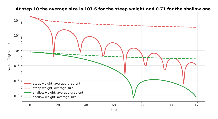
Two solid and two dashed lines on a log scale, showing the average gradient and the average size for the steep and the shallow weight

At step 10 the average size is 107.617 for the steep weight and 0.713 for the shallow one, which is what each weight's step is divided by.

Dividing by the usual size of a weight's own gradient is what buys the per-weight step size, and the two moves then come out close to each other.

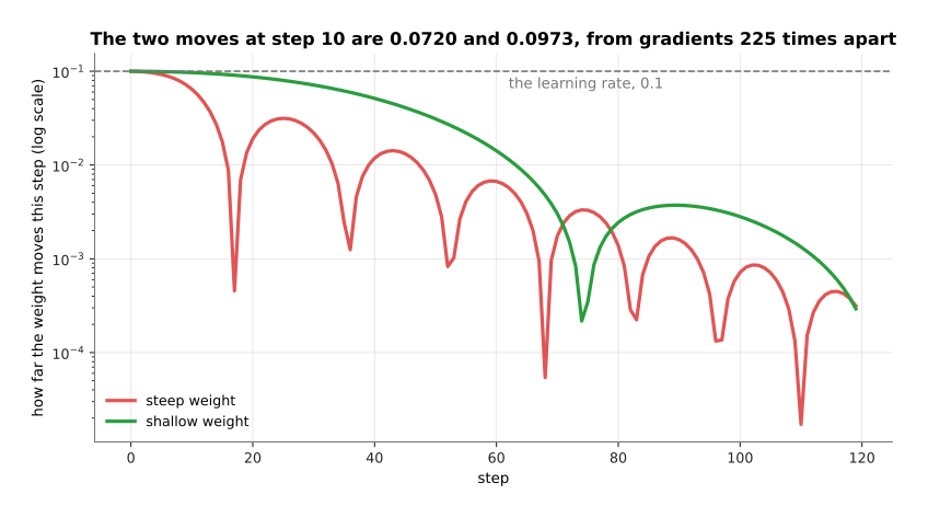
Two lines on a log scale of how far each weight moves at each step, both starting at the learning rate of 0.1

At step 10 the steep weight moves -0.0720 and the shallow one moves -0.0973, which is within a factor of 0.74 of each other, although the two gradients started 225 times apart.

A weight whose gradients are large gets a small step, and a weight whose gradients are tiny gets a large one. The learning rate then stops meaning a distance, and starts meaning roughly how far any weight may move in one step. That is why one learning rate often works across very different networks, and it is the main reason Adam is the default almost everywhere.

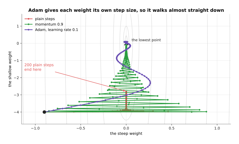
A contour map of the same valley with three paths from the same start, for plain steps, momentum, and Adam

After 200 steps on the same problem the plain rule has reached a loss of 7.811e-01, momentum 3.138e-04, and Adam 2.050e-08.

What Adam costs is memory, because it stores two numbers per weight instead of momentum's one. The optimiser's state is then twice the size of the model itself.

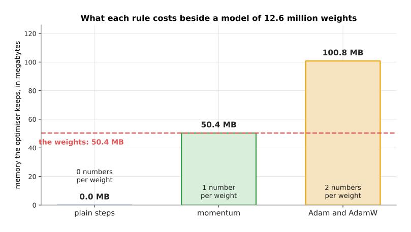
A bar chart of the memory three optimiser rules keep beside a model of 12.6 million weights, at 0, 50.4 and 100.8 megabytes

Beside a model of 12,595,200 weights, which is 50.4 megabytes, plain steps keep nothing, momentum keeps 50.4 megabytes and Adam keeps 100.8 megabytes.

Those 100.8 megabytes are the 0.10 gigabytes in the memory picture of backpropagation. Adam also has two settings for how long its two averages remember, usually 0.9 and 0.999, and a small number added to the square root so that nothing is divided by zero.

There is one more piece, and it is the difference between Adam and the version that almost everyone now uses. Training often includes weight decay, which shrinks every weight slightly towards zero at every step, because weights that stay small tend to give a network that works better on examples it has not seen. The old way of applying weight decay was to add a term to the gradient. With Adam that goes wrong, because the added term is then divided by the square root of the second average, along with everything else.

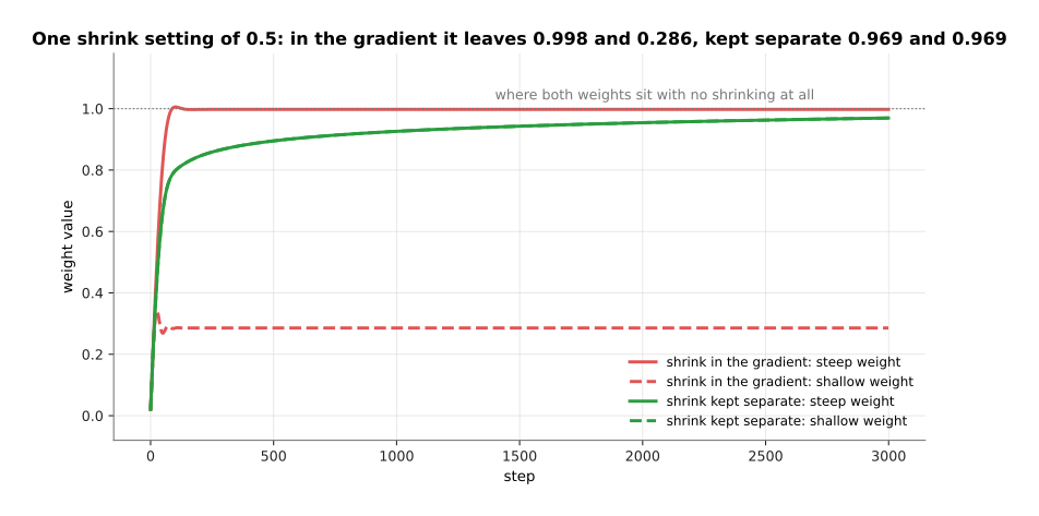
Four weight paths over 3000 steps, where three settle near 1.0 and the one with the shrink inside the gradient settles near 0.29

Both weights should settle at 1.0, and with a shrink setting of 0.5 added to the gradient the steep weight ends at 0.9975 while the shallow one is dragged down to 0.2857; with the shrink kept separate both end at 0.9695.

Read that picture as two weights that should both settle at 1.0. Adding the shrink to the gradient means that a weight with large gradients barely feels the shrink, because its division is large, while a weight with small gradients is pulled almost to nothing. So one setting does two completely different things inside the same network. AdamW is Adam with the shrinking taken out of the gradient and applied directly to the weight after the step is taken.

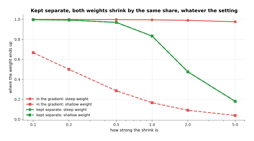
Four lines of where each weight ends up against the strength of the shrink, where the two kept-separate lines lie exactly on top of each other

Kept separate, both weights end at the same value for every setting, from 0.997 at a shrink of 0.1 down to 0.180 at a shrink of 5.0, while added to the gradient the two weights end far apart at every setting.

Every weight keeps the same share of itself, whatever its gradients look like, so the setting means one thing across the whole network. That is the whole difference between Adam and AdamW, and it is why AdamW rather than Adam is what modern models are trained with.

4. Learning-rate schedules and warmup#

The last two sections changed how the gradient becomes a step. This section changes the learning rate itself, which neither of them touched. Keeping the rate at one value for a whole run is the obvious thing to do, and it is not the best thing to do, because what you want early in a run and what you want late in it are different. A plan for changing the learning rate as the run goes along is called a schedule.

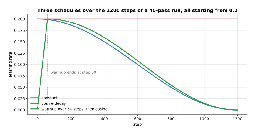
Three curves of learning rate against step over 1200 steps, one flat, one falling as a cosine, and one rising for 60 steps before falling

All three schedules are built from a top rate of 0.2: the constant one stays there, the cosine one is at 0.1000 halfway and 0.00000 at the end, and the third starts at 0.0033 and spends its first 60 steps climbing to the top rate before following the same curve down.

The falling shape is called cosine decay, after the curve it follows. Its reason is that a large rate early covers ground quickly, while a small rate late lets the weights settle instead of bouncing around the bottom. The rising part at the start is called warmup, and it exists because the first few steps are the most dangerous in the whole run.

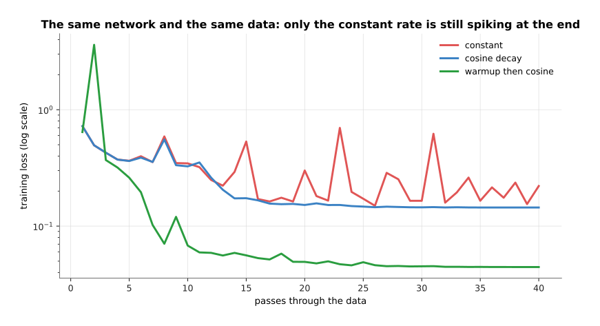
The training loss of three runs over 40 passes on a log scale, with the constant run spiking again and again

On the same network and the same data, the constant rate is still spiking at pass 40, while the cosine run and the warmup run have both settled.

The spikes are the point. A rate that is large enough to make progress early is too large to sit still at the end, so the constant run never settles. Decay removes the spikes, because the rate at the end is small. What the two runs are worth is best read at the end of the run, on the held-back examples.

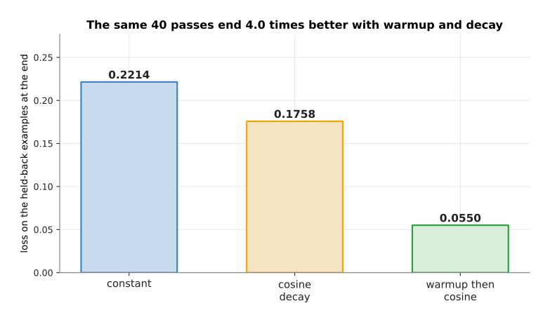
A bar chart of the final held-back loss of the three runs, at 0.2214, 0.1758 and 0.0550

After the same 40 passes, a constant rate of 0.2 ends with a held-back loss of 0.2214, cosine decay ends at 0.1758, and warmup followed by cosine decay ends at 0.0550, which is 4.0 times better than the constant run.

Warmup earns its place most clearly when the rate is too large to start with at all.

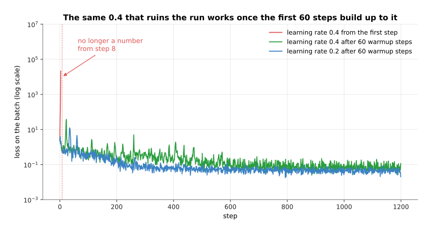
A chart of the batch loss over 1200 steps for three runs, one of which shoots up and stops after eight steps

A flat learning rate of 0.4 makes the loss stop being a number at step 8, while the same 0.4 reached through 60 warmup steps trains normally and ends at a held-back loss of 0.0770.

The obvious alternative to warmup is to use a rate that is safe from the first step, which here would be 0.2, and that run is the blue line, which also works. What warmup buys is that you may use rates that would otherwise be impossible. That matters most for large models, where a bigger rate is worth a lot and the first steps are the ones most likely to destroy the run. What warmup costs is one more setting to choose, which is how many steps the warmup lasts.

5. Where the weights start#

Warmup protects the first steps. This section is about what those first steps start from, because a network's weights have to hold some value before the first forward pass can run. Choosing those values is called initialisation, and the rule is that they are random but not arbitrary.

The random part is not an accident of laziness, and the two pictures below show what happens without it.

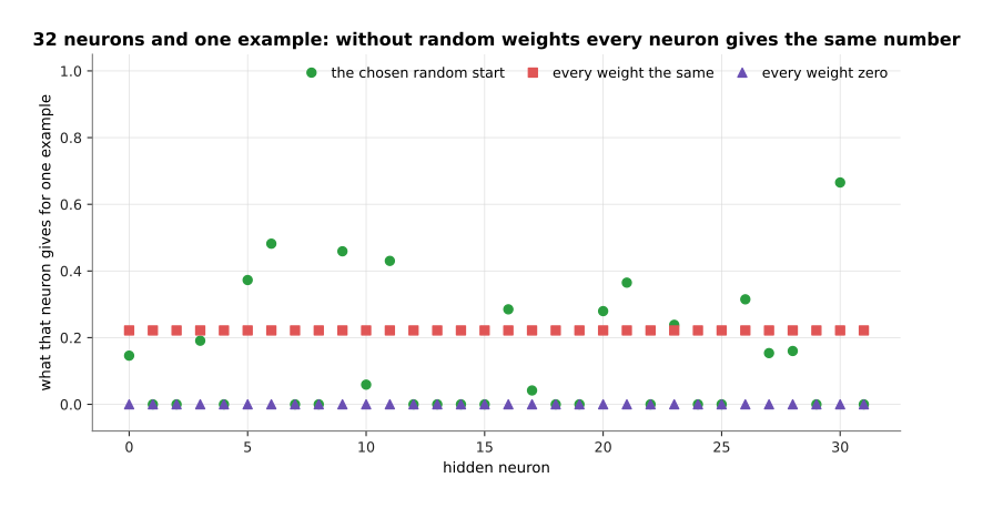
A chart of what each of 32 hidden neurons gives for one example, under three starting schemes

With every weight set to zero all 32 hidden neurons give 0.0, with every weight set to the same value they all give 0.2217, and only the random start spreads them out, from 0.000 to 0.665.

Giving every neuron the same output is already bad. What makes it permanent is that the backward pass then hands every neuron the same gradient.

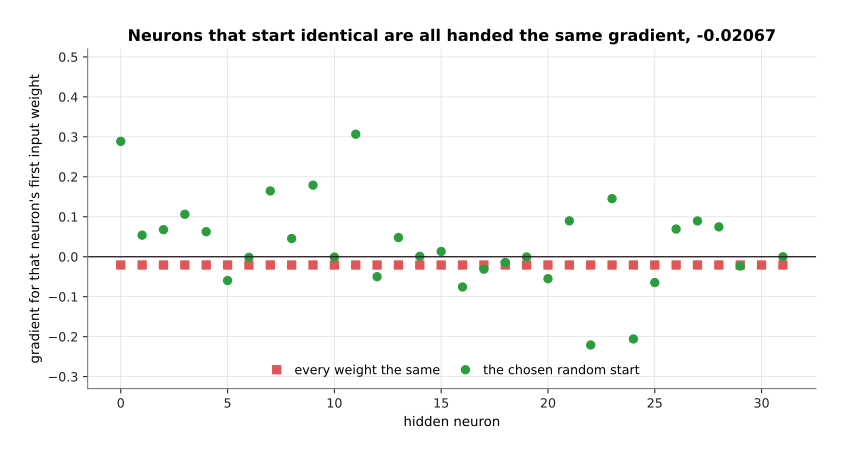
A chart of the gradient each of the 32 neurons is handed for its first input weight, under two starting schemes

With every weight the same, all 32 neurons are handed a gradient of exactly -0.02067, while the random start hands out 32 different values.

Setting every weight to zero kills the network outright, because each hidden neuron gives 0, the output never depends on any hidden weight, and every hidden gradient is 0 for ever. Setting every weight to the same value that is not zero is only slightly better. Neurons that start identical are handed identical gradients, so they take identical steps and stay identical, and a layer of 32 of them does exactly as much work as one neuron would. Random values break that tie, and breaking the tie is their entire job.

The part that is not arbitrary is the size of those random values, because that size decides the size of the numbers running through the network on the very first batch. Read the picture below as three measurements of the first batch, taken at three starting sizes, on a scale where each line of the grid is ten times the one below it.

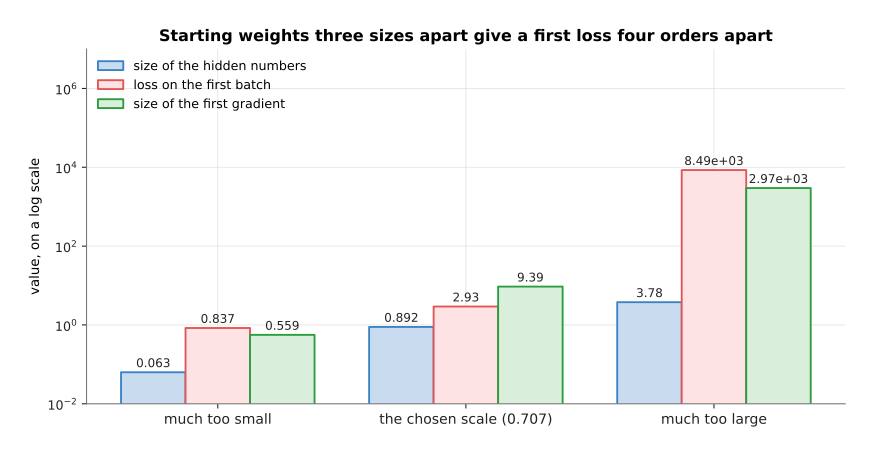
A grouped bar chart on a log scale showing the hidden number size, the first loss and the first gradient for three starting scales

Starting weights that are much too small give hidden numbers of 0.063 and a first loss of 0.837, the chosen scale gives 0.892 and 2.93, and weights that are much too large give 3.78 and a first loss of 8491.

The chosen scale here is 0.707, and it is not a guess. It is calculated from the number of inputs a neuron has, so that the numbers coming out of a layer are about the same size as the numbers going into it. That is the same balance that backpropagation showed holding the blame level on the way back. Every framework has this built in, so you get it without asking for it.

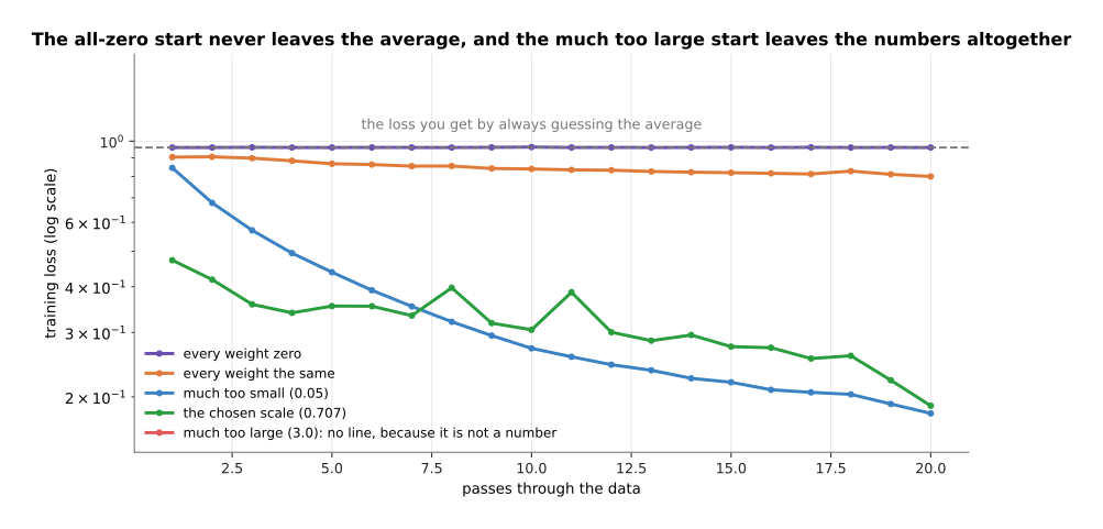
Five loss curves over 20 passes, with the zero start flat on a dashed line and the chosen scale falling fastest at the start

The all-zero start sits at 0.9607 for the whole run, which is exactly the loss you get by always guessing the average of the targets, the all-the-same start reaches only 0.8006, and the much too large start is not a number at all, so it has no line.

Two of those five lines deserve an honest word. The much too large start does not merely train badly. Its first gradient is 2970, which throws the weights so far that the loss stops being a number, and that is the exploding gradient of the page before happening on step one. The much too small start, on the other hand, trains perfectly well here. It ends at 0.1802 against the chosen scale's 0.1891, and that is not a mistake. This network has one hidden layer, so there is nothing for a small scale to shrink away through. Give the same small scale fifty layers and it becomes the red line from the page before, which arrives with nothing left.

6. Reading the curve, the time a run takes, and the checkpoint#

Everything so far was a decision made before the run starts. This last section is about the run itself, which produces one picture that you have to be able to read. That picture is the loss drawn against the passes through the data, with one line for the training examples and one line for the held-back ones.

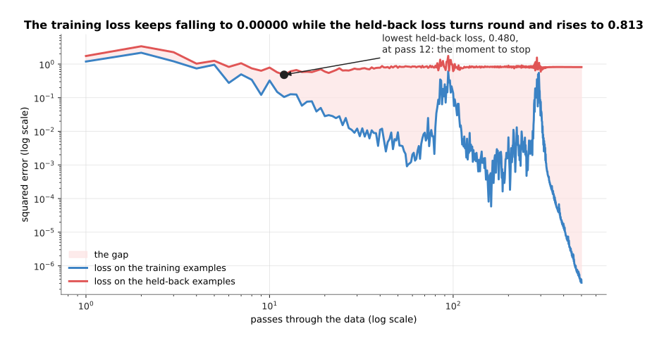
A chart on log axes of training loss and held-back loss over 500 passes, with the gap between them shaded and the lowest held-back point marked

The training loss falls all the way from 1.191 to 0.00000, while the held-back loss reaches its lowest point of 0.480 at pass 12 and then climbs back to 0.813 by pass 500.

The gap opening between those two lines is the single most important shape in training. The run that drew it was set up to make the shape obvious, with a training set cut down to 24 examples and a network far too large for them. The training loss keeps falling because the network is learning those 24 examples by heart. The held-back loss rises because knowing 24 examples by heart is of no use on anything else. Where the two lines part company is where a run stops being worth continuing, which is the subject of the next chapter's overfitting and generalisation.

Three other shapes come up often enough to be worth recognising on sight. The first one is the shape of a run with nothing wrong with it.

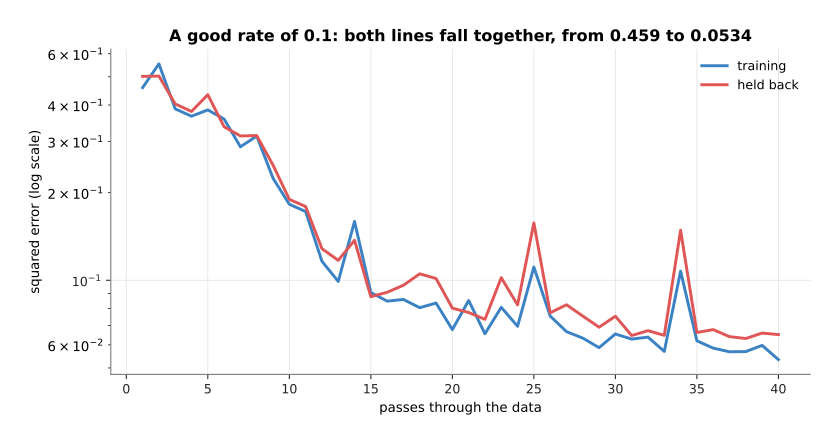
A training curve and a held-back curve over 40 passes, both falling together to about 0.05

A good rate of 0.1 takes the training loss from 0.459 to 0.0534, and the two lines stay together all the way.

Two lines falling together and flattening mean that nothing is wrong, and that the run may simply need more passes. The second shape is slower and smoother.

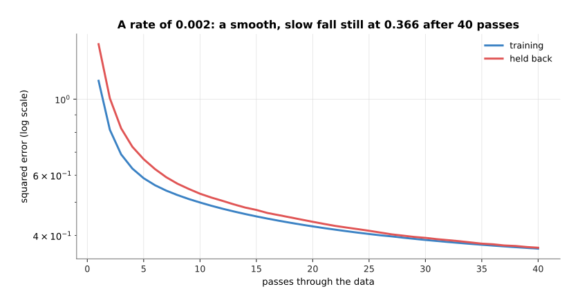
A training curve and a held-back curve over 40 passes, falling smoothly and still well above 0.3 at the end

A rate of 0.002 is still at 0.366 after 40 passes, and the curve has not begun to flatten.

A smooth fall that has not flattened by the end of the run means the learning rate is too small. The run would get there eventually, so this is a waste of time rather than a failure. The third shape is the opposite.

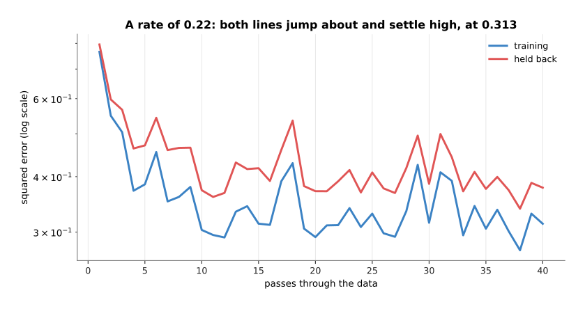
A training curve and a held-back curve over 40 passes, both jumping up and down and settling around 0.3

A rate of 0.22 makes both lines jump about from pass to pass, and the training loss settles high, at 0.313.

A line that jumps about and settles high means the rate is too large. That is told apart from the shape in the first picture of this section by the held-back line: here the held-back line jumps about, and there it climbed steadily away from the training line.

How long any of this takes is the number of steps multiplied by the time of one step, and the time of one step is set by how much arithmetic the step is.

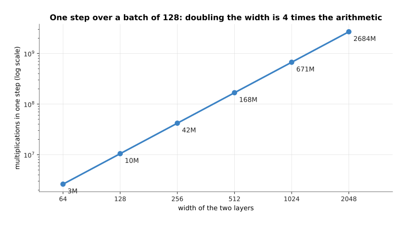
A line on log axes of multiplications in one step against the width of the network, rising by a factor of four each time the width doubles

One step over a batch of 128 is 2,621,440 multiplications at width 64 and 2,684,354,560 at width 2048, because doubling the width makes one step four times as much arithmetic.

Those counts cover the forward pass and the backward pass together, which comes to two and a half multiplications for every weight and every example in the batch. Turning arithmetic into seconds depends on the machine, so the honest way to answer the question for your own run is to time one step and multiply.

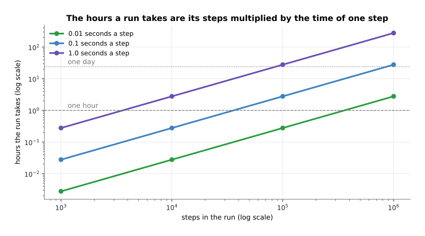
Three lines on log axes of hours against steps in the run, for three speeds per step, with dashed lines at one hour and one day

At a tenth of a second a step, 10,000 steps take 0.28 hours and 1,000,000 steps take 27.78 hours, and at a whole second a step those same two runs take 2.78 and 277.78 hours.

Small models finish in minutes. The fine-tuning runs that most people do take hours. The largest models are trained for weeks on many machines at once. So a run that you cannot afford to lose is a normal thing to have, and that is what the last line of section 1 was for. A checkpoint is a file holding the weights as they stood at some point in the run. It is written at the end of each pass, so that a run which stops for any reason can be continued rather than started again.

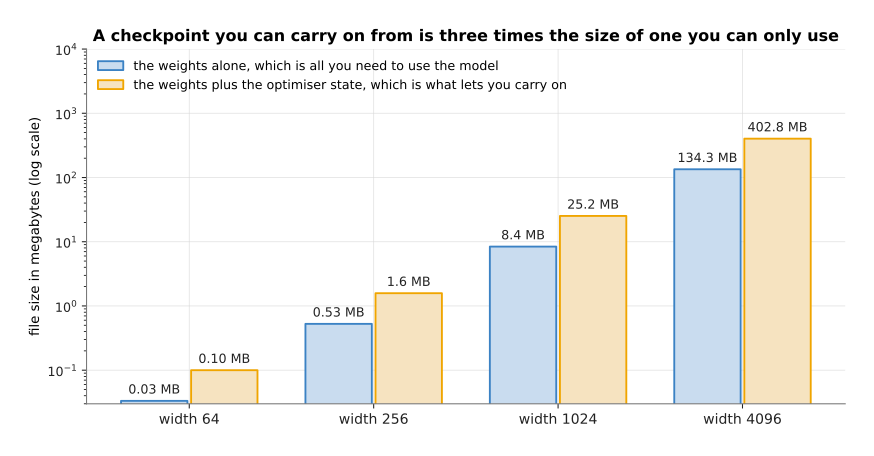
A bar chart on a log scale of checkpoint size against network width, with one bar for the weights alone and one for the weights plus the optimiser state

A two-layer network of width 1024 has 2,099,200 weights, which is 8.40 megabytes on their own and 25.19 megabytes once the optimiser's two running averages are saved beside them.

The difference between those two bars is the difference between the two jobs a checkpoint does. If you only want to use the model, the weights are all you need. If you want to carry the run on from where it stopped, you also need the optimiser state from section 3, which is two more numbers for every weight and so three times the file size.

7. Where to read next#

Overfitting and generalisation is the next page, and it takes up the gap in section 6's curve: what memorising is, how the held-back set is built, and when to stop.
Normalisation and stability explains the loss spikes of section 4 and the layer-by-layer rescaling that makes large runs survive.
Backpropagation is the page before this one, and it is where line 4 of the loop comes from.
Scale, data and compute takes section 6's arithmetic up to the size of real training runs, and explains what a graphics processing unit does with it.
Fine-tuning in the catalogue book is this loop applied to a real robot model, with the settings people actually use.

8. Using it in Python#

Section 1 wrote the loop out in seven lines, and in PyTorch those seven lines are seven lines. This is the whole of this page in one block, with the optimiser of section 3, the schedule of section 4 and the checkpoint of section 6 in their proper places.

import torch
from torch import nn

model = nn.Sequential(nn.Linear(4, 32), nn.ReLU(), nn.Linear(32, 1))
opt = torch.optim.AdamW(model.parameters(), lr=0.01, weight_decay=0.01)  # section 3
steps_per_epoch, epochs = 30, 20                                         # section 1
warm = torch.optim.lr_scheduler.LinearLR(opt, 0.01, 1.0, total_iters=60)
cos = torch.optim.lr_scheduler.CosineAnnealingLR(opt, T_max=540)
sched = torch.optim.lr_scheduler.SequentialLR(opt, [warm, cos], [60])    # section 4

# A stand-in for your own data, so that this block runs as it stands: 960
# examples of four readings and one answer, which is 30 batches of 32.
x = torch.randn(960, 4)
y = x @ torch.tensor([1.5, -0.8, 0.3, 2.0]) + 0.1 * torch.randn(960)
loader = torch.utils.data.DataLoader(
    torch.utils.data.TensorDataset(x, y), batch_size=32, shuffle=True)

for epoch in range(epochs):
    for x, y in loader:                 # line 1: loader hands out batches of 32
        out = model(x)                  # line 2: the forward pass
        loss = ((out[:, 0] - y) ** 2).mean()   # line 3: the loss for this batch
        loss.backward()                 # line 4: the backward pass
        opt.step()                      # line 5: the optimiser moves every weight
        opt.zero_grad()                 # line 6: or the next batch adds to these
        sched.step()                    # line 7 follows: on to the next batch
    torch.save({'model': model.state_dict(),
                'opt': opt.state_dict()}, f'checkpoint-{epoch}.pt')      # section 6

The library gives you the optimiser, the schedule and the saving. AdamW holds the two running averages of section 3 for every weight and applies the weight decay separately. Adam is the same class with the older behaviour that section 3 advised against. The two schedulers joined by SequentialLR are the warmup and the cosine decay of section 4, which is why total_iters=60 and T_max=540 add up to the 600 steps of section 1. The starting weights of section 5 are already chosen sensibly inside nn.Linear.

You still have to decide the learning rate, which no library can pick for you, and the batch size, which sets both the memory used and how noisy each step's gradient is. You decide how long the warmup lasts and how many steps the whole run has, and T_max has to match the second of those, or the rate will reach zero at the wrong time. You also decide what goes into the checkpoint. The code above saves both the model and the optimiser state, which is the larger of the two bars in the last picture and the one that lets a stopped run carry on.

One last thing: the loop above has no evaluation in it beyond the loss it trains on, and no real run is like that. The held-back loss of section 6 belongs at the end of each epoch, inside with torch.no_grad(): so that no tape is kept, and the next chapter is about what you do with the number it gives you.