Starting a Model of Your Own — The order of the work

The page before this one, before you train anything, ends with two things written down. The first is the job, set out as an input, an output and one number that says whether it worked. The second is a baseline, which is the simplest answer you could use instead of a model, and which the model has to beat before anybody may call its score evidence. This page is about the day after that. It is about the order of the work, rather than about any one method.

The order matters because a model can fail for a dozen different reasons, and those reasons cost wildly different amounts to find. Some of them show up in a single pass of one batch through the model, with no training at all. Others show up only in a run that takes a week. So the work is done in four milestones, starting with the cheapest. This page calls them rungs, in the way that a ladder has rungs, because each one stands on the one below it and you climb them in order. Each rung rules out a group of causes, so that a failure on the next rung has a short list of suspects. The four rungs are these: put one batch through the untrained model and read the loss; make the model memorise ten examples on purpose; do one small honest run with a held-back set; and only then make things bigger, one change at a time.

The page assumes three things from earlier pages. It assumes the loop from the training loop, which is the cycle of taking a batch, measuring the loss, and changing the weights. It assumes the loss from the score of being wrong, and in particular cross-entropy, which is the loss used when the model has to choose one of several classes. It assumes the held-back set from overfitting and generalisation, which is the group of examples the model never trains on. What this page adds is what to look at, what the number should be before you look at it, and what each result rules out.

Every number here was measured. The data is simulated. One example is sixteen readings, standing in for features already pulled out of a camera frame, and its label is one of ten classes. Enough noise is added that the ten classes overlap, so the job is possible but not easy. A pool of 2,200 examples was drawn once, and 600 of them were set aside as the held-back set before any training happened. Everything done to that pool is real PyTorch, and docs/diagrams/starting_your_own_model_2.py prints every figure quoted below.

Contents#

The ladder, and why the cheapest rung comes first
Rung one: one batch through an untrained model
Rung two: memorise ten examples on purpose
Rung three: one small honest run
Rung four: scale, one change at a time
The run folder, and the run you keep
Where to read next
Using it in Python

1. The ladder, and why the cheapest rung comes first#

The job and the baseline say nothing about what to do first. So this section sets the four rungs out and measures what each one costs, counted in example-views. One example-view is one example put through the model once, and it is the thing that takes the time, because every one of them is arithmetic the machine has to do.

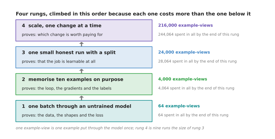
Four stacked boxes for the four rungs, each with what it proves and the number of example-views it costs, with arrows pointing upwards and the running total beside each one

The four rungs cost 64, 4,000, 24,000 and 216,000 example-views, so 244,064 have been spent by the time the fourth one ends.

Read that picture from the bottom. One batch of 64 examples through an untrained model costs 64 example-views. It proves that the data arrives, that the shapes line up and that the loss starts where it should. Four hundred steps on the same ten examples costs 4,000 example-views, and it proves that the loop, the gradients and the labels work together. A run over 960 examples for 25 passes costs 24,000 example-views, and it is the first run that can say whether the job is learnable at all. Nine runs of that size cost 216,000 example-views, which is nearly nine tenths of the whole total.

The order follows from those four numbers, because the same fault costs a different amount depending on which rung finds it.

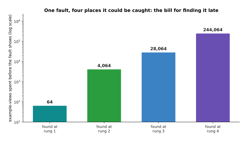
A bar chart on a log scale of the example-views spent before a fault shows, rising from 64 at rung one to 244,064 at rung four

The same fault found on the fourth rung has cost 244,064 example-views instead of 64, which is 3,814 times as much work for the same answer.

Those numbers count arithmetic rather than minutes, because minutes depend on the hardware, and this page knows nothing about your hardware. The ratio is what matters. Catching an input that never reaches the output on the second rung costs 4,064 example-views, and catching the same fault on the fourth costs 244,064, which is sixty times as much.

The rungs are also worth climbing in order because of what each one rules out. The next picture lists thirteen faults that really happen and marks the first rung that catches each one.

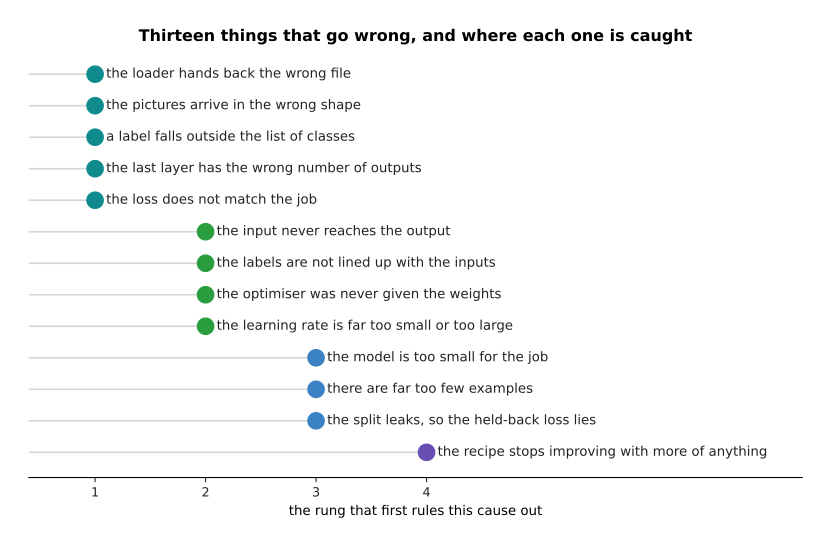
Thirteen named faults, each with a marker at the rung that first catches it, from the loader handing back the wrong file at rung one to the recipe no longer improving at rung four

A label outside the list of classes, and a last layer with the wrong number of outputs, both show on the very first batch. Three other faults survive the first rung and are caught on the second: the input never reaching the output, the labels not being lined up with the inputs, and the optimiser never having been given the weights.

So if you are on the fourth rung wondering why the loss will not fall, the answer is almost never something that the first two rungs would have caught. The next picture counts the same thirteen causes a different way, as the number still open after each rung.

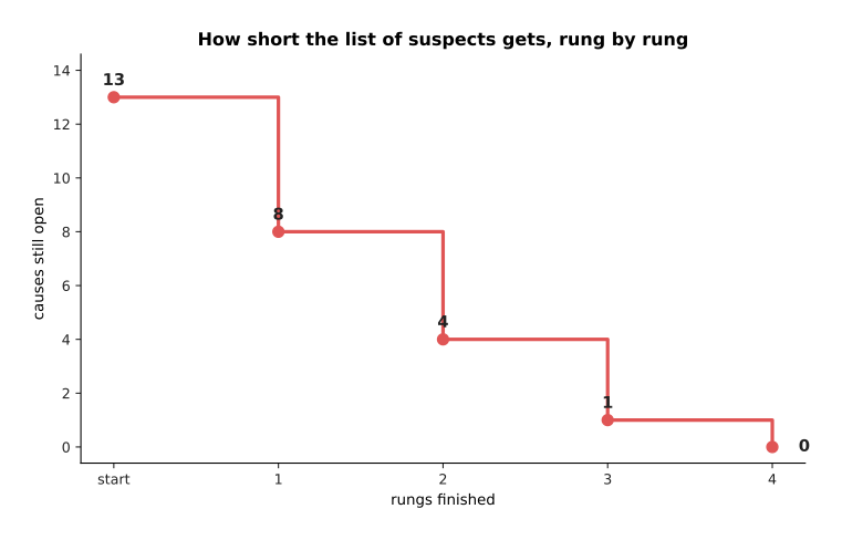
A step chart of the number of causes still open, falling from thirteen before any rung to eight, four, one and zero

Of the thirteen faults, five are ruled out on the first rung, four more on the second and three more on the third, so the number still open falls from 13 to 8 to 4 to 1.

That falling number is the whole argument for the order. Each rung is cheap compared with the one above it, and each one shortens the list of things you have to think about when the next one fails.

2. Rung one: one batch through an untrained model#

The first rung costs one forward pass, which is one batch travelling through the model from the input to the output, with no weights changed. Most people skip it, which is why it is the most useful check on this page. You put one batch through the model before any training, and you look at two things: the shape of what comes out, and the loss. The loss is no mystery, because you can work out in advance what it has to be.

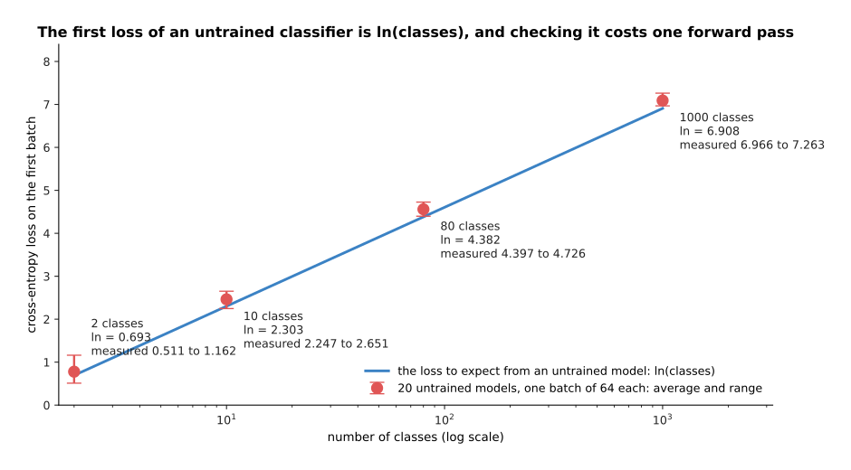
A chart of cross-entropy loss against number of classes on a log x axis, with the curve of the natural logarithm drawn through measured points at 2, 10, 80 and 1000 classes, each with the range over twenty untrained models

Twenty untrained models give losses between 0.511 and 1.162 on a job with 2 classes, where the expected value is 0.693. On 10 classes they give 2.247 to 2.651, against an expected 2.303. On 80 classes they give 4.397 to 4.726, against 4.382. On 1000 classes they give 6.966 to 7.263, against 6.908.

Here is where those expected values come from. A model that knows nothing spreads its belief evenly, so it gives each class a probability of one divided by the number of classes. The cross-entropy of that spread is the natural logarithm of the number of classes. The natural logarithm answers the question "to what power must 2.71828 be raised to give this number", and you do not need to know more than that here. It gives 2.303 for ten classes, 6.908 for a thousand, and 0.693 for a two-way choice. The measured values sit near those lines rather than exactly on them, because random starting weights give a model mild opinions that it did not earn. So a first loss within a few tenths of the expected value is healthy, and a first loss of 11 on a ten-class job is a bug.

The other thing to read off the first batch is the shape of what comes out. A shape is the list of sizes of a block of numbers, so a shape of (8, 10) means eight rows of ten numbers. The next picture follows one real batch through a small picture model and prints the shape after every layer.

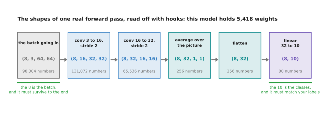
Six boxes in a row showing the shape and the number of values after each layer of a small convolutional network, from the batch going in to the ten class scores coming out

One real forward pass goes from (8, 3, 64, 64), which is 98,304 numbers, through (8, 16, 32, 32) and (8, 32, 16, 16), down to (8, 32) and finally to (8, 10). The model holds 5,418 weights.

Two of those numbers matter, and they are marked in green. The first number in each shape is the batch, which is 8 here, and it must still be 8 at the end, because a layer that loses it has mixed your examples together. The last number is the count of classes, which is 10 here, and it must match the number of different labels in your data. A model with eleven outputs and ten labels trains happily and is wrong in a way that no loss curve shows.

Now for the faults this rung catches. The next picture takes one untrained model, plants a different bug in each copy of it, and reads the first loss off each copy.

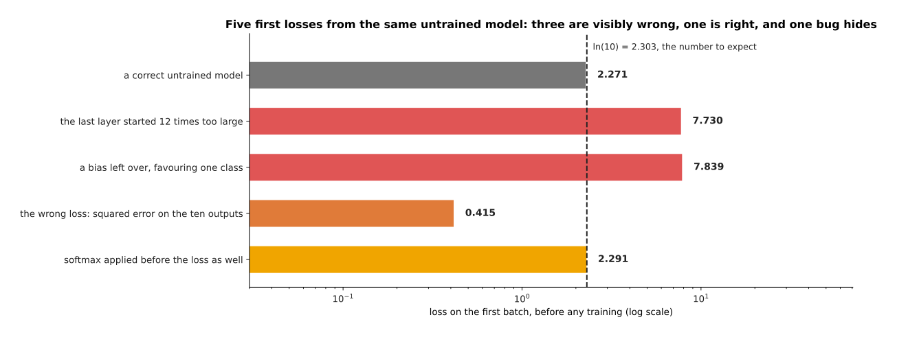
A horizontal bar chart on a log scale of five first losses from the same untrained model, with a dashed line at ln(10)

A correct untrained model gives 2.271. A last layer whose weights started twelve times too large gives 7.730. A bias left over from something else, favouring one class, gives 7.839. The wrong loss, which here is squared error on the ten outputs, gives 0.415.

The two values near 7.8 are the easiest to spot. Weights that start too large make the model certain of answers it has no reason to believe, and cross-entropy charges most for being certain about a wrong answer. The value of 0.415 sits below the expected loss instead, because squared error on ten outputs is a different quantity altogether, with no reason to land near 2.303. The last bar is the honest warning. A softmax applied by hand before a loss that applies its own softmax gives 2.291, which is nearer to 2.303 than the correct model is. A softmax turns raw scores into probabilities that add up to one, and applying it twice is a real and common bug. This rung cannot catch it, so the next rung has to.

The same check works for a job that predicts a number rather than a class, but the value to expect is different. The next picture shows the same first-batch measurement twice: once with the target left in millimetres, and once with the same target centred and scaled.

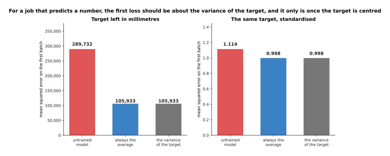
Two bar charts of mean squared error on the first batch, one with the target in millimetres and one with the same target standardised, each showing the untrained model, always guessing the average, and the variance of the target

With the target left in millimetres, the untrained model scores 289,732 against a variance of 105,933. With the same target standardised, it scores 1.114 against a variance of 0.998.

For a job that predicts a number, compare the first loss against the variance of the target. The variance is the average of the squared distances from the average, and it is what you score by always guessing the average. The left panel shows what happens when the target keeps its own units. The untrained model starts near zero, while the targets average 428.7 millimetres, so most of the first loss is that gap squared, which is 183,809 on its own. That is not a bug in itself, but it makes any real bug impossible to see beside it, and that is why targets are centred and scaled before training.

3. Rung two: memorise ten examples on purpose#

The first rung proved that the data goes in with the right shape, and it said nothing about whether training does anything at all. So the second rung is the smallest experiment that does. You train on ten examples over and over, and you demand that the loss fall to nearly zero. This is the most useful hour in the whole process, because a model that cannot memorise ten examples will not learn ten thousand, and finding that out costs 4,000 example-views instead of a week.

Choose one example of each class for this test, as the runs below do. Ten examples drawn at random prove much less, and the next picture says why.

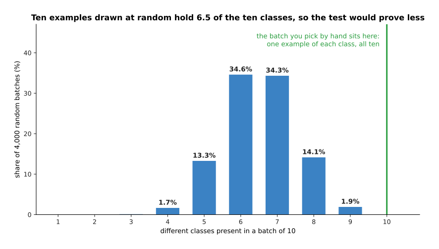
A bar chart of how many of the ten classes appear in a batch of ten drawn at random, peaking at six and seven classes and never reaching ten

Over 4,000 batches of ten drawn at random, a batch holds 6.5 of the ten classes on average. The most common results are six classes, in 34.6 per cent of batches, and seven classes, in 34.3 per cent. Not one of the 4,000 batches held all ten.

So a random batch of ten leaves three or four classes untested, and the test then says nothing about whether the model can separate those. Picking one example of each class by hand costs a minute and removes that hole. The next picture runs the test itself: the same ten examples, 400 times, for three different models.

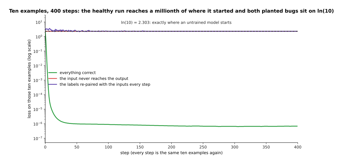
A chart on a log scale of the loss over 400 steps for three runs on the same ten examples, one falling to about a millionth and two sitting on a dashed line at ln(10)

The healthy run starts at 2.553, is below 0.0001 by step 6, and ends at 6.795e-07, which is about seven ten-millionths. The run with the input zeroed and the run with the labels re-paired with the inputs on every step both sit exactly on 2.303.

The green line is what passing looks like, and the difference between it and the other two is large. Both flat lines land on 2.303, which is the natural logarithm of ten, and that is precisely where an untrained model starts. That is no coincidence. A model that cannot see the input, or whose labels are shuffled against the inputs on every step, can do no better than give every class the same probability. So a flat line at exactly the first loss says that nothing in the input is reaching the answer.

The loss is not the only thing to watch. The next picture counts how many of the ten examples each run gets right, and adds a fourth run whose labels were shuffled once and then left alone.

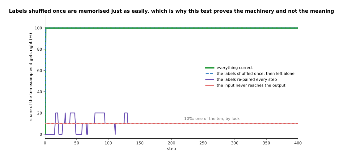
A chart of the share of ten examples got right over 400 steps for four runs, with two reaching 100 per cent and two staying at 10 per cent

The correct run and the run whose labels were shuffled once both go to 100 per cent right after a single step. The two broken runs stay at 10 per cent, which is one of the ten by luck.

Shuffling the labels once does not stop the model memorising them, because memorising is all this test asks for, and a wrong answer is as easy to memorise as a right one. That is why this rung proves the machinery and not the meaning. It says that gradients flow, that the optimiser is connected to the weights, and that the model can separate these ten examples. It says nothing about whether your labels are right. Wrong labels show up on the third rung instead.

A flat line tells you that something is broken, and the next picture tells you what. It draws the ten-by-ten table of probabilities that each run ends up giving the ten examples. Each row is one example and each column is one class, so a healthy run should have one dark square in each row.

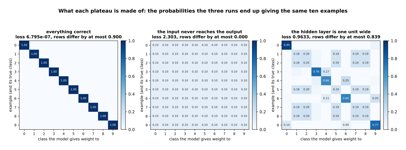
Three heatmaps of the ten-by-ten table of probabilities each run ends up giving the ten examples, one a clean diagonal, one every cell at 0.10, and one a partial diagonal

The healthy run gives 1.0000 to the right class every time. The run with the input cut off gives 0.1000 to every class, and its rows differ from each other by 0.0000. A model with a hidden layer of one unit gets 60 per cent right and ends at a loss of 0.9633.

The middle panel is the pattern worth memorising, because every row equals every other row to four decimal places. The model is giving the same answer whatever it is shown, and nothing except a broken connection does that. The right panel is a different failure. A hidden layer of one unit can separate examples along a single direction only, so it gets some of them right and gives the rest a mixture of answers. That is a model too small for the job rather than a bug, and the picture tells the two apart where the loss alone would not.

The next picture collects seven single-batch runs and their final losses, so that each failure can be recognised by its number alone.

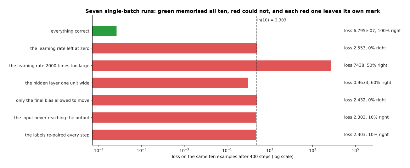
A horizontal bar chart on a log scale of the final loss of seven single-batch runs, with the one that memorised all ten in green and six that did not in red

The correct run ends at 6.795e-07. A learning rate of zero stays at its first loss of 2.553. A learning rate 2000 times too large ends at 7438. A hidden layer one unit wide ends at 0.9633. A run in which only the final bias may move ends at 2.432. The two runs with no connection from the input end at 2.303.

Three of those leave a mark you can recognise with no other evidence. A learning rate of zero leaves the loss at exactly the first batch's value, which is a perfectly flat line. A learning rate far too large ends far above the logarithm of the number of classes, which is worse than knowing nothing, and that happens only when each step moves the weights much too far. A flat line at exactly the logarithm means one answer for everything. An hour spent here buys you four suspects instead of thirteen.

The claim underneath this whole rung is that a model which fails here will fail later too. The next picture measures that claim. It takes the same model at six different widths, runs the ten-example test on each, and then runs each one properly on 240 examples.

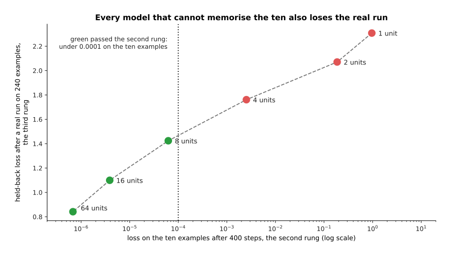
A scatter of the loss on ten examples against the held-back loss of a real run, for hidden layers of 1, 2, 4, 8, 16 and 64 units, rising from left to right

A hidden layer of 1 unit ends at 0.9633 on the ten examples and at a held-back loss of 2.308 on the real run. Two units give 0.1864 and 2.071, four units give 0.002527 and 1.761, eight units give 0.00006233 and 1.424, sixteen units give 0.000003886 and 1.100, and sixty-four units give 6.795e-07 and 0.842.

The order is the same on both rungs, and the one-unit model is worse than useless on the real run, because 2.308 is above the 2.303 that an untrained model scores. So the cheap test ranks the models in the same order as the expensive one, which is exactly what it is for.

4. Rung three: one small honest run#

The second rung proved that the machinery works on ten examples. Memorising ten examples is not learning, so the third rung is the first run that uses the split decided on the page before. It trains on 960 examples in batches of 32 for 25 passes, which is 750 steps, and after each pass it measures the loss on the 600 examples it never trains on.

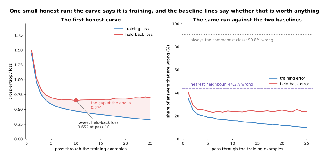
Two panels, one with the training and held-back loss over 25 passes and the gap between them shaded, and one with the error rates of the same run against two baseline lines

The training loss falls from 1.435 to 0.322, and the held-back loss falls from 1.494 to a lowest point of 0.652 at pass 10 and then rises slightly to 0.697. At the end, 23.8 per cent of held-back answers are wrong, against 44.2 per cent for nearest neighbour and 90.8 per cent for always answering the commonest class.

The left panel on its own only says that the loss went down. The right panel answers the question the page before set, because the dashed lines are the baselines, and the model is worth something only below them. It is worth something here, since 23.8 per cent wrong against nearest neighbour's 44.2 per cent is a gap the simple method cannot close. Had the held-back line settled at 46 per cent, the run would have failed while showing a perfectly healthy-looking loss curve, and that is why the baselines are drawn on the chart.

The gap between the two curves is itself a measurement. The next picture runs the same recipe on three sizes of training set and writes the final gap beside each pair of curves.

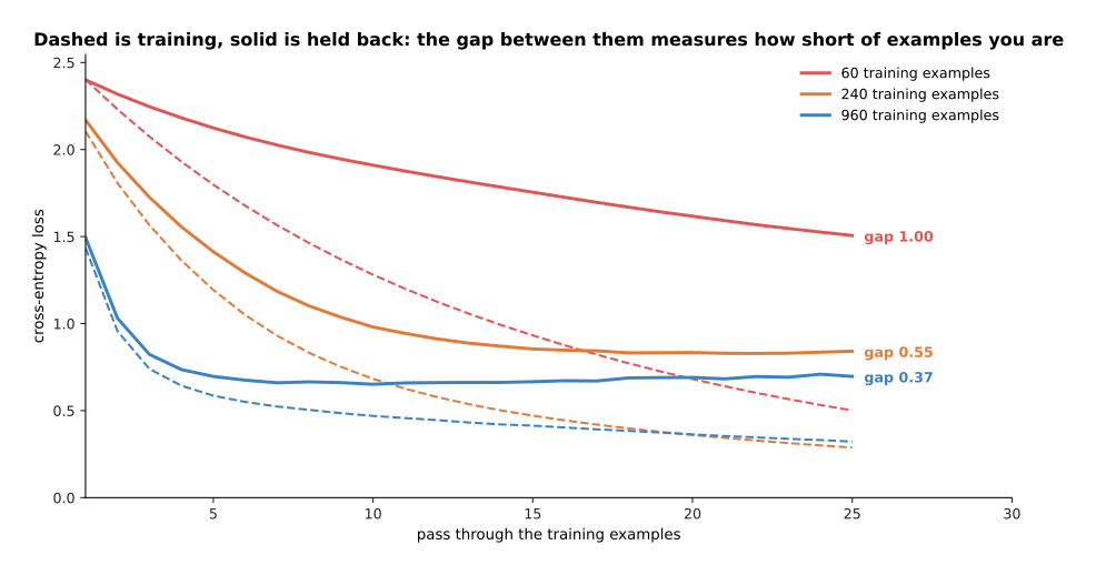
Three pairs of curves, dashed for training and solid for held back, for runs on 60, 240 and 960 examples, with the end gap written beside each pair

With 60 training examples the gap at the end is 1.00 and 48.0 per cent of held-back answers are wrong. With 240 examples the gap is 0.55 and 28.3 per cent are wrong. With 960 examples the gap is 0.37 and 23.8 per cent are wrong.

The training loss is low in all three runs, because a model with enough weights fits whatever is put in front of it. So the held-back loss is what separates them. A wide gap that keeps closing as examples are added is the clearest sign that the next thing to buy is data rather than a bigger model, and here multiplying the examples by four twice took the gap from 1.00 to 0.55 to 0.37. The 60-example run was also still falling at pass 25, while the 960-example run had flattened by pass 10, so a number of passes that suits one size does not suit another.

One fault can make all of this look better than it is. The next picture repeats the 240-example run twice: once with a clean split, and once with a split in which half the held-back rows are copies of training rows.

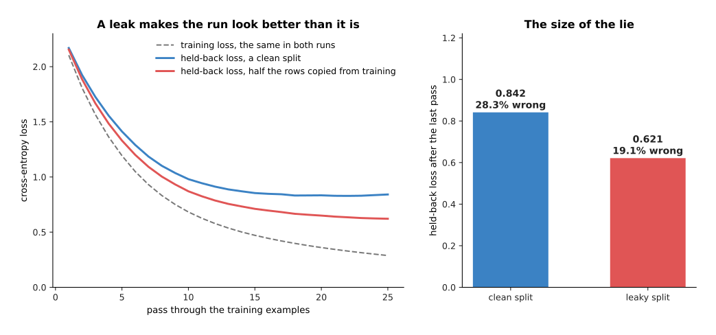
Two panels, one with the training loss and two held-back curves for a clean and a leaky split, and one with a bar for each final held-back loss

The clean split ends at a held-back loss of 0.842, with 28.3 per cent of answers wrong. The leaky split ends at 0.621, with 19.1 per cent wrong.

A leak is an example that is in the held-back set and in the training set at the same time. The leak planted here is obvious, and it makes the run look better by 0.220 of loss and by 9.3 points of error. Real leaks are harder to see, and they move the number in the same direction: two camera frames a tenth of a second apart, one object photographed twice, one demonstration counted as several examples. That is why overfitting and generalisation insists that the split be made along whatever line groups those near-copies, made once, written down, and never made again by another piece of code.

Most first runs come back with one of four shapes, and the shape says what to do next. The next picture shows all four, each from a real run on this job.

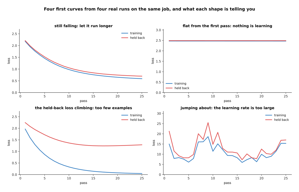
Four small panels of training and held-back loss curves, labelled still falling, flat from the first pass, held-back loss climbing, and jumping about

The still-falling run ends at 0.591 on training and 0.699 on held back. The flat run sits at 2.469 and 2.488 from the first pass onwards. The run on 60 examples reaches 0.046 on training while its held-back loss climbs to 1.286. The fourth run jumps about, and its held-back loss reaches 25.496 at its worst.

Two lines falling together means that nothing is wrong and the run should be longer. Two flat lines from the first pass mean that nothing is learning, and after the second rung you already know that this is a learning rate near zero rather than a disconnected model. A training loss near zero with a held-back loss climbing means the model is memorising, and the cure is more examples or a smaller model. A curve that jumps by tens means a learning rate far too large, and the size of the numbers on the axis gives that away at a glance.

5. Rung four: scale, one change at a time#

The third rung gave one run that works and one number that beats the baseline, which is the first point at which making anything bigger makes sense. The fourth rung is a sequence of runs with one rule: each run changes one thing from the run before it. The measurements below are what happens when that rule is kept, and then what happens when it is broken.

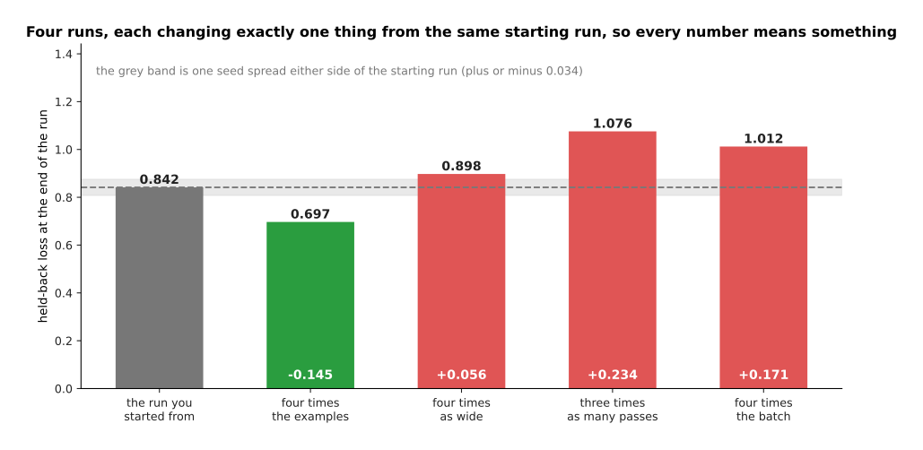
A bar chart of the final held-back loss of a starting run and four runs that each change one thing, with the change written inside each bar and a grey band for the seed spread

The starting run ends at a held-back loss of 0.842. Four times the examples gives 0.697. Four times the width gives 0.898. Three times as many passes gives 1.076. Four times the batch gives 1.012.

Each of those runs is readable because exactly one thing moved. Four times the examples is worth 0.145 of loss, and it is the only change here that helps. Three times as many passes costs 0.234, because this run was already past its best point at pass 10. Four times the batch costs 0.171, because the same passes with a bigger batch mean a quarter as many steps, and a step is where the weights actually change. Four times the width moves the answer by 0.056, which is too small to call a result, for the reason given two pictures below.

The next picture breaks the rule on purpose. It takes one change that helps and one that hurts, and makes both at once.

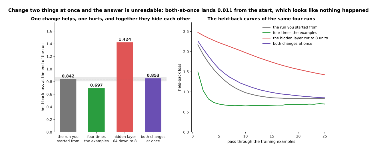
Two panels, one with bars for a starting run, two single changes and both changes together, and one with the held-back curves of the same four runs

Four times the examples takes the loss from 0.842 down to 0.697. Cutting the hidden layer from 64 units to 8 takes it up to 1.424. Doing both at once gives 0.853, which is 0.011 away from where it started.

That is the demonstration. One of those changes was worth having, the other made the model much worse, and the run that made both came back saying that nothing had happened. Somebody who changed two things and saw no change would conclude that neither mattered, and would be wrong twice over. Nothing about the combined run is faulty. The number 0.853 simply cannot be attributed to anything, because two effects of opposite sign landed on top of each other.

Before believing any of those differences, you need to know how much a run moves on its own. The next picture runs the same settings six times, changing only the seed.

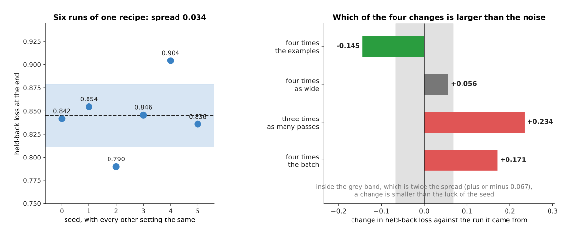
Two panels, one showing the final held-back loss of six runs of identical settings with different seeds, and one showing the four single changes against a band of twice that spread

Six runs with identical settings, differing only in the seed, end at 0.842, 0.854, 0.790, 0.846, 0.904 and 0.836. Their spread is 0.034, and the difference between the best and the worst is 0.115.

A seed is the number that decides every random choice a run makes, which here means the starting weights and the order the examples are shuffled into. Six runs that differ only in the seed land 0.115 apart. So any change smaller than that is luck rather than progress, and twice the spread, which is 0.067, is a reasonable line to draw. By that line, three of the four changes above are real, and the wider model at 0.056 is not. The honest report for a change inside the band is that you cannot tell, and two or three seeds of each setting settle it cheaply.

The rule of one change at a time has a cost, and it is worth seeing what the alternative costs. The next picture counts the runs each approach needs, on a logarithmic scale, because the two counts end up thousands apart.

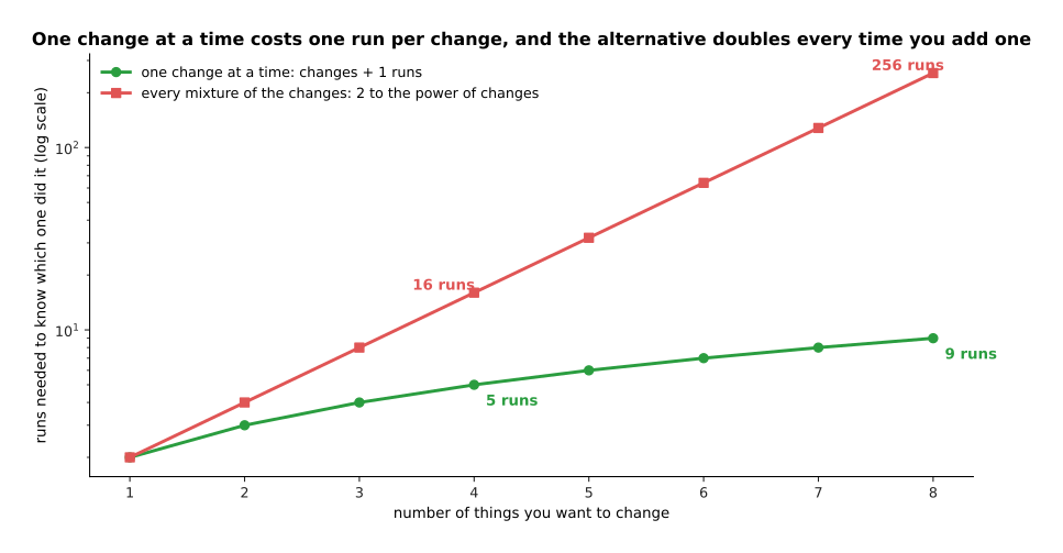
A chart on a log scale of the number of runs needed against the number of things you want to change, with one line for one change at a time and one for every mixture

Telling eight changes apart takes 9 runs when they are made one at a time, and 256 runs when every mixture of them is tried. At 6,000 example-views a run, those are 54,000 and 1,536,000 example-views.

The obvious alternative is to try every combination. It does find effects that appear only when two settings move together, and it costs 2 raised to the power of the number of changes. For eight changes that is 256 runs, and at the size of a real training job that is not a week anybody has. So people change one setting, keep the winner, and move on, accepting that a pair of settings which only works jointly will be missed. That is a real cost, and it is the price of an answer you can read.

6. The run folder, and the run you keep#

The fourth rung produces many runs, and a folder of runs is worth nothing unless you can say which settings produced which number. So this section is about what to write down. Its rule is that the run you keep is not the one with the best number, but the one you can do again.

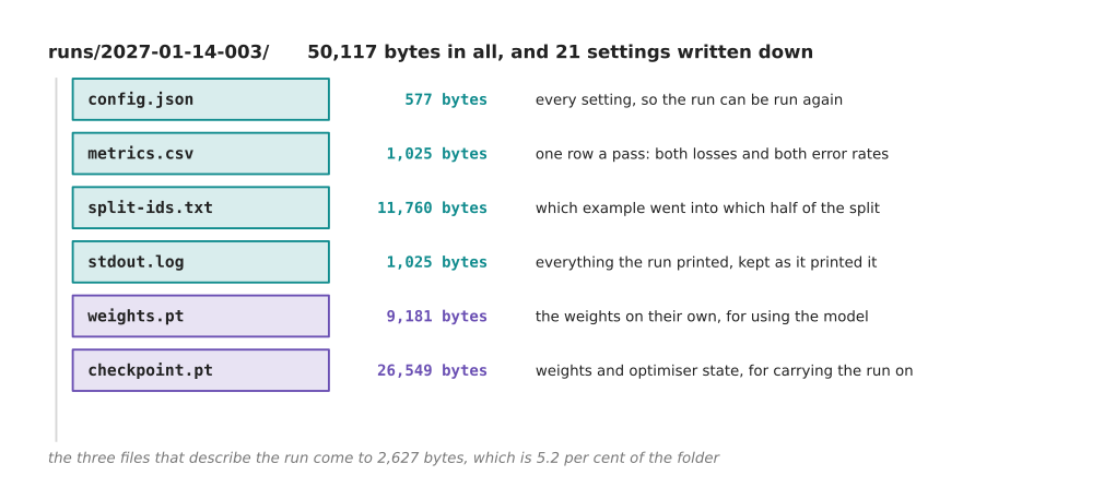
A drawing of a run folder listing six files with their real byte sizes and a note on what each one is for

A real run folder holds config.json at 577 bytes, metrics.csv at 1,025 bytes, split-ids.txt at 11,760 bytes, stdout.log at 1,025 bytes, weights.pt at 9,181 bytes and checkpoint.pt at 26,549 bytes, which is 50,117 bytes in all.

Those six files are a good minimum, and the first one carries most of the value, because it holds all 21 settings the run used. The metrics file has one row per pass, so a curve can be drawn again without running anything again. The list of which example went into which half of the split stops the split quietly changing between runs. The last two files are the model saved twice: once as the weights alone, for using the model, and once together with the optimiser state, for carrying the run on later, as the training loop explains.

The seed belongs in that config file, and the next picture shows what it buys. It runs the same settings twice with the same seed, and then twice with different seeds.

Two panels, one with two curves from the same settings and the same seed lying exactly on top of each other, and one with two curves from the same settings and different seeds

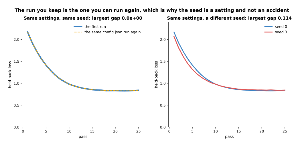
Running the same settings with the same seed twice gives two curves whose largest difference is 0.0e+00, which means they are identical. A different seed gives curves that differ by as much as 0.114 and end at 0.842 against 0.846.

The left panel is what reproducible means in practice. The second run lands on the first to the last digit the computer keeps, and that happens only because the seed was written down with everything else. A folder without a seed holds a run you can repeat approximately, and that is not the same thing when you are looking for a difference of 0.05.

Not every setting matters equally, and the next picture sorts them by how far changing one moves the final answer. The grey band is twice the seed spread, so a bar that stays inside it has moved the answer less than luck does.

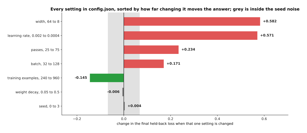
A horizontal bar chart of how far the final held-back loss moves when each setting is changed one at a time, sorted by size, with a grey band for the seed noise

Cutting the width from 64 to 8 costs 0.582 and dropping the learning rate from 0.002 to 0.0004 costs 0.571. Tripling the passes costs 0.234 and quadrupling the batch costs 0.171. Four times the examples gains 0.145. Changing the weight decay and changing the seed move the answer by 0.006 and 0.004.

The two settings at the top would make a run unrecognisable if they were lost, and the learning rate in particular is why a run folder with no config file is barely a result at all. The two at the bottom land inside the seed band. That does not mean they can be left out, because a setting that does not matter on this job may matter on the next one, and writing it down costs one line.

The last question is what all this writing down costs, and the next picture answers it in bytes, on a logarithmic scale.

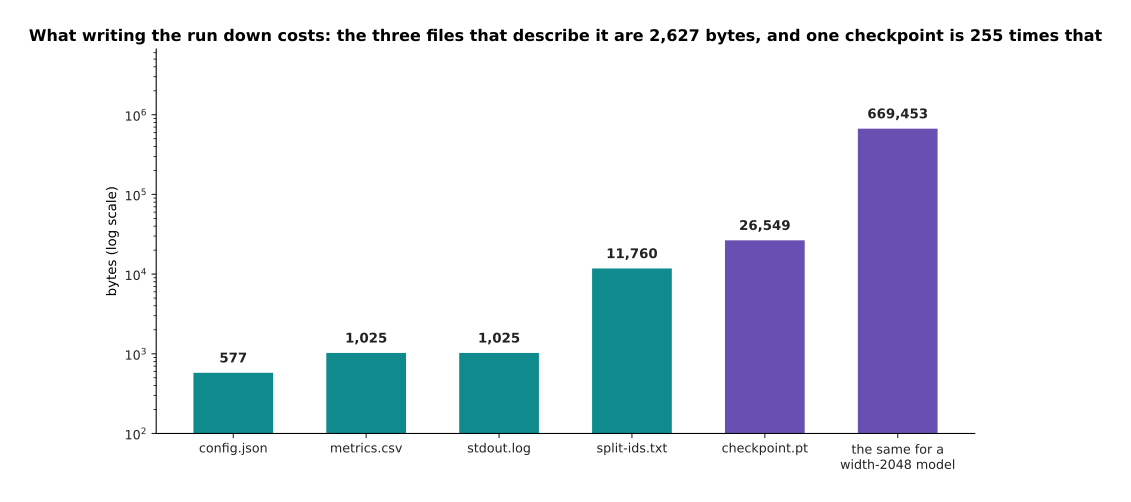
A bar chart on a log scale of the byte sizes of four text files, a small checkpoint and the checkpoint of a wider model

The three files that describe the run come to 2,627 bytes. A checkpoint of a model with 55,306 weights is 669,453 bytes, which is 255 times as much.

So writing down what a run was costs 2,627 bytes against the 669,453 bytes of one checkpoint, which is less than half of one per cent. Real models are far larger than this one, so that share only gets smaller. There is no version of this in which logging is the expensive part. What is expensive is a folder of twelve runs with no way of telling which one produced the number you liked, and the cure is to write the settings down before the run rather than after it.

7. Where to read next#

What to reuse and what to train is the next page, and it decides what the model on rung three should actually be, from using somebody else's model as it is through to training from nothing.
Before you train anything is the page this one follows, and it is where the job, the baseline and the split that rung three depends on are decided.
When it does not work is the diagnosis page, and it picks up where the four rungs end, with the failures that survive all of them.
Overfitting and generalisation explains the gap in section 4 properly, and how a split is built so that it cannot leak.
The training loop is where the loop, the optimiser and the checkpoint of section 6 come from.
Evaluation and failure in the catalogue book is what the fourth rung becomes once the model is on a real arm, where the number to beat is counted in trials rather than in loss.

8. Using it in Python#

The first two rungs are about twenty lines of PyTorch between them, and this is all of it. The block runs as it stands on ten made-up examples. It prints the check from section 2, and both the test and the planted bug from section 3, so that passing and failing appear side by side.

import json
import pathlib

import torch
from torch import nn
import torch.nn.functional as F

torch.manual_seed(0)
x = torch.randn(10, 16)                      # ten examples, sixteen readings each
y = torch.arange(10)                         # section 3: one example of each class
model = nn.Sequential(nn.Linear(16, 64), nn.ReLU(), nn.Linear(64, 10))

# Section 2: one batch through the untrained model, before any training at all.
with torch.no_grad():
    out = model(x)
    first = F.cross_entropy(out, y)
print('what comes out has shape', tuple(out.shape))
print('first loss %.3f, and ln(10) is %.3f' % (first, torch.tensor(10.0).log()))

# Section 3: memorise those ten on purpose. If this will not fall, stop here.
opt = torch.optim.AdamW(model.parameters(), lr=0.05)
for _step in range(200):
    loss = F.cross_entropy(model(x), y)
    opt.zero_grad()
    loss.backward()
    opt.step()
print('after 200 steps on ten examples, loss %.2e' % loss.item())

# Section 3 again, with the input cut off, which is the bug the test catches.
broken = nn.Sequential(nn.Linear(16, 64), nn.ReLU(), nn.Linear(64, 10))
opt = torch.optim.AdamW(broken.parameters(), lr=0.05)
for _step in range(200):
    loss = F.cross_entropy(broken(torch.zeros_like(x)), y)
    opt.zero_grad()
    loss.backward()
    opt.step()
print('with the input zeroed, loss %.3f' % loss.item())

# Section 6: write the settings down before the run, not after it.
cfg = {'seed': 0, 'learning_rate': 0.05, 'steps': 200, 'batch': 10, 'classes': 10}
pathlib.Path('config.json').write_text(json.dumps(cfg, indent=2) + '\n')
print('config.json is', pathlib.Path('config.json').stat().st_size, 'bytes')

That block prints a shape of (10, 10), a first loss of 2.332 against an expected 2.303, a loss of 4.17e-07 after 200 steps, a loss of 2.303 for the run whose input was zeroed, and a config file of 89 bytes. Those five numbers are the whole of the first two rungs, and the only part to change for your own job is the line that makes x and y.

The library gives you very little of this, and that is the point. PyTorch will not tell you that your first loss is wrong, because it does not know how many classes you meant to have. F.cross_entropy will cheerfully accept probabilities where it wanted raw scores, and hand back a number that looks fine. Nothing in the library will tell you that a model cannot memorise ten examples either, because from the library's side nothing failed.

What you still choose is the ten examples, and one of each class is worth having, because section 3 measured that a random ten holds only 6.5 of the ten classes. You choose the number of steps, and a few hundred is plenty, since a model that will memorise ten examples usually does it in under fifty. You also choose what goes in the config file, and the rule from section 6 is that anything you would have to guess in order to repeat the run belongs in it, with the seed first.