The page before this one, Normalisation and stability, ended by saying that the numbers given to a network have to be scaled, so that training stays steady. That page assumed that the input was already a list of numbers. Every page before it assumed the same thing. This chapter asks where those numbers come from, because nothing a robot meets arrives as a list of numbers on its own. A sentence is made of letters. A photo is made of light. The arm's own readings are angles and forces, measured in units that have nothing to do with each other.
This page does that job for text. Text is the clearest case, and everything else copies its pattern. The page answers four questions. How is a sentence cut into pieces? How does a piece become a list of numbers? What does it mean for two of those lists to be near each other? How does a model find out what order the pieces came in? By the end you will be able to read the input stage of any language model and say what each part is for. The page assumes that you know what a weight is, what a layer is, and what training does. It assumes nothing at all about language.
The text behind the numbers here is invented. The script
turning_the_world_into_numbers.py
writes 3,200 short robot instructions from a set of sentence patterns. It then
builds a small tokeniser and a small table of word vectors from those
instructions. The methods are the real ones, and they are applied in full to
that text, so every count and every similarity below is a genuine output of the
script. What is small here is the scale. A real tokeniser is built from a vast
amount of text and holds tens of thousands of pieces, so it cuts words into
fewer pieces than this one does.
Contents#
- A token is a piece of text the model treats as one unit
- Why pieces, and not whole words or single letters
- The embedding table is a lookup
- Near each other means used in the same way
- Telling the model what order the tokens came in
- What the picture of the geometry leaves out
- Where to read next
- Using it in Python
1. A token is a piece of text the model treats as one unit#
A network takes numbers as its input, and it takes a fixed quantity of them. A sentence is made of letters, so the first job is to cut the sentence into pieces that can be counted and numbered.
A token is one such piece of text. The model treats a token as a single unit, and it never looks inside it. The program that does the cutting is called a tokeniser. The list of every piece that the tokeniser is allowed to produce is called its vocabulary. Each piece has a place in that list, and the number of that place is the piece's number. That number is the only thing the model ever receives.
The picture below shows one instruction before and after the cutting. The row of boxes is the list of tokens, and the small number under each box is that token's place in the vocabulary.
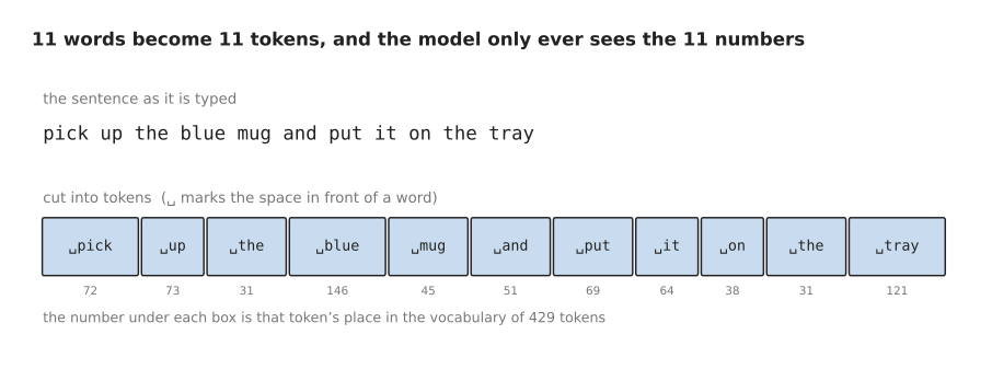
The instruction is cut into eleven tokens, and the vocabulary that these tokens come from holds 429 pieces in all.
The open box character ␣ stands for the space in front of a word. The tokeniser keeps that space inside the token. This means the tokeniser can rebuild the original sentence exactly, spaces included.
Every one of those eleven words is common in the text the tokeniser was built from. Because of that, each word became a single token. The model therefore receives the numbers 72, 73, 31, 146, 45, 51, 69, 64, 38, 31 and 121. The number 31 appears twice, because the word "the" appears twice. Words that are not common behave differently, and the next picture shows how.
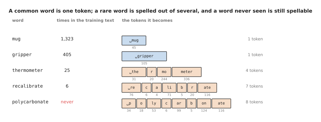
A word the tokeniser saw often gets a token of its own. A rare word is spelled out of smaller pieces. A word the tokeniser never saw can still be spelled.
The word "mug" appeared 1,323 times in the training text, so it earned a token of its own. The word "gripper" appeared 405 times, so it earned one too. The word "thermometer" appeared only 25 times, so it is spelled with four pieces instead. The word "polycarbonate" never appeared at all, and it is still spelled, using eight pieces that do exist.
This method is called subword tokenisation. The word "subword" means that a piece may be part of a word rather than a whole word. Because any word can be spelled from smaller pieces, the model can read a word that nobody showed it during training. However, the method also means that the number of tokens in a sentence is not the number of words in it. That matters, because everything a model costs is counted in tokens.
The next picture counts five robot instructions in three ways. Read each group of three bars as one instruction. The green bar is the number of whole words, the blue bar is the number of subword tokens, and the grey bar is the number of single letters.
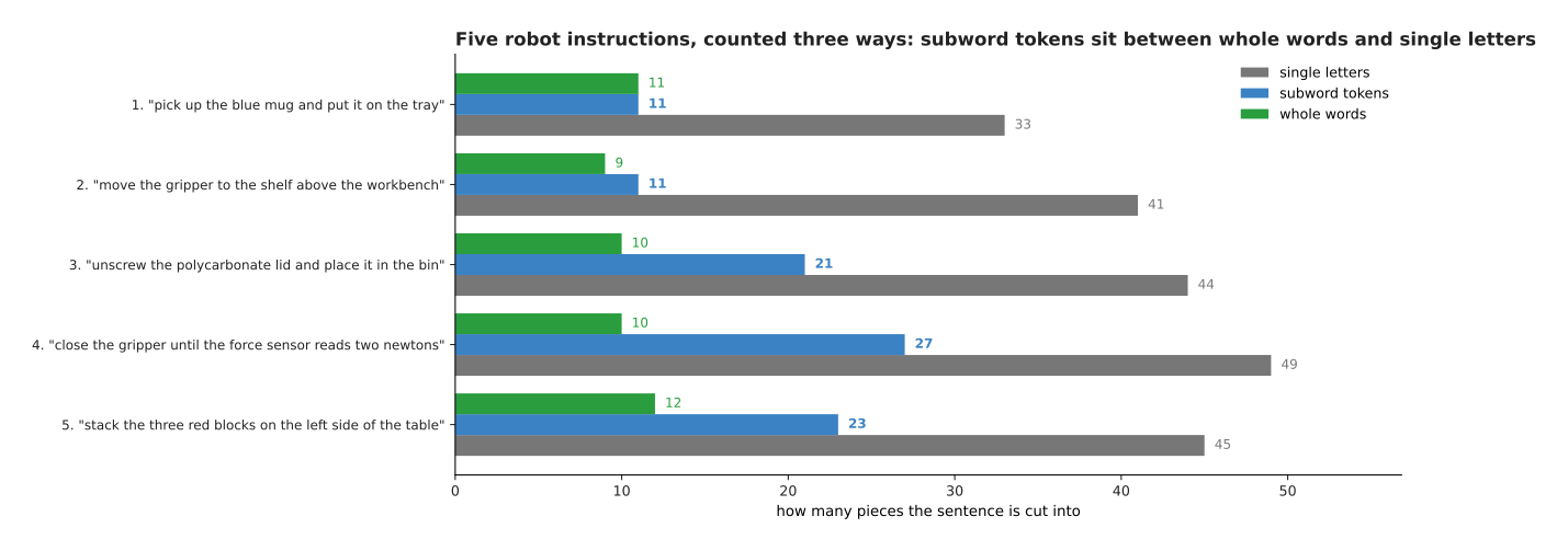
For every one of the five instructions, the subword count sits between the word count and the letter count.
The first instruction has eleven words and eleven tokens, because every word in it is common. The fourth instruction has ten words and twenty-seven tokens, because it contains six words that the training text never used: "until", "force", "sensor", "reads", "two" and "newtons". Across all five instructions there are 52 words, 93 tokens and 212 letters, which is 1.79 tokens for every word. The next section explains why the pieces are chosen in this way, rather than in either of the two obvious alternative ways.
2. Why pieces, and not whole words or single letters#
Subword pieces look like a strange compromise, so this section measures what the two simpler choices would cost. The first choice is to give every whole word its own token. The second choice is to give every single letter its own token.
The next picture splits one instruction in all three ways. Each row is one way of splitting, and the count at the end of a row is how many tokens that way produces.
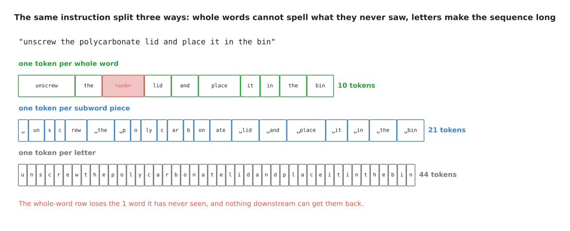
The same instruction is split three ways, and the whole-word row loses the one word that the tokeniser has never seen.
A whole-word vocabulary gives the shortest sequence, which is ten tokens here, and that is its only advantage. The cost is shown by the red box. The word "polycarbonate" is not in the vocabulary, so the tokeniser has nothing to give the model except a single "unknown" token. Every other unseen word becomes that same "unknown" token. The model therefore cannot tell a polycarbonate lid from a titanium one, and it cannot spell either word back out, because the information was thrown away before the model ever ran. Robot work is full of part names and measurements, so unseen words appear constantly.
Single letters have the opposite problem. A letter vocabulary never fails, because every word is made of letters that the vocabulary already holds. The sequence, though, is more than four times as long: 44 tokens instead of 10. Length is expensive for a transformer. The attention step described in Attention compares every token with every other token, so doubling the length makes that step about four times as much work.
Subword pieces combine the advantage of each choice. Common words stay whole, and anything unusual is spelled from smaller pieces. How short the sequence becomes then depends on how many pieces the vocabulary holds, and the next picture measures that.
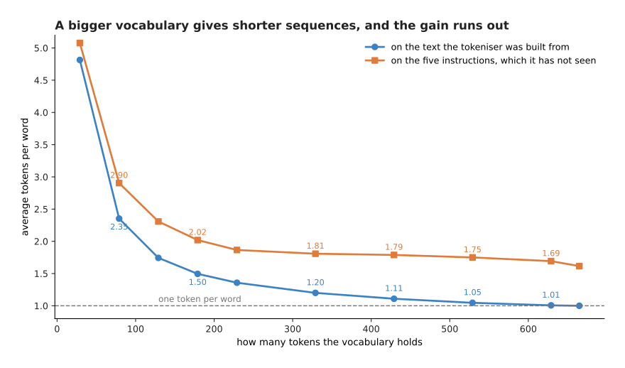
A bigger vocabulary gives shorter sequences, and most of the gain has already been collected by about 200 tokens.
With an alphabet alone, which is 29 tokens in all, it takes 4.81 tokens to write the average word. That falls to 1.74 at a vocabulary of 129 tokens, to 1.20 at 329 tokens, and to exactly 1.00 at 665 tokens, where no further merging is possible. The fall from 4.81 to 1.00 is a fall of 3.81, and 3.46 of that has already happened by 229 tokens, which is about nine tenths of the whole gain.
So the gains become small quickly. Meanwhile the embedding table described in the next section grows in direct proportion to the vocabulary. Real models balance those two costs against each other. A common vocabulary size today is between about 30,000 and 150,000 pieces, and a few models use more than 250,000.
The way the pieces are chosen is called byte pair encoding, and the method is simpler than the name. The tokeniser starts with every word written out as single characters. It then counts every pair of neighbouring pieces across the whole training text. It joins the most common pair everywhere that pair appears, which adds one new piece to the vocabulary. It then repeats the count and the join, so each round adds exactly one piece.
The table below lists the first ten pairs that this tokeniser joined. Read each row as one round: the rank says which round it was, the pair is what was joined, the new token is the result, and the last column is how often that pair appeared when it was chosen.
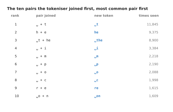
The pairs are joined in order of how often they appear, so the most common pair is joined first.
The first pair joined is a space and the letter "t", which appeared 11,845 times. The second joins "h" and "e" into "he", which appeared 9,375 times. The third joins the results of the first two into the whole word "the", which appeared 8,900 times.
Those merges are then applied, in the same order, to any word the tokeniser is asked to cut. The next picture follows one word through that process. Each row is the state of the word after one more merge has been applied, and the number on the right is how many pieces are left.
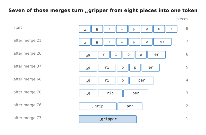
The word "gripper" starts as eight separate characters, and seven merges turn it into a single token.
The merges that do this work are the ones numbered 21, 26, 37, 68, 70, 76 and 77. Nothing in this process chooses meaningful units, because the only rule is how often a pair appears next to each other. That is why "thermometer" is split into "the", "r", "mo" and "meter", rather than into anything a person would call parts of a word. Once the pieces exist, each piece needs numbers of its own, and those numbers live in the embedding table.
3. The embedding table is a lookup#
A token number such as 45 is a name, not a measurement. Giving it to a network directly would be wrong, because 45 is not three times as much of anything as 15 is. What the model needs instead is a list of numbers for each token, and those numbers must be ones the model can do arithmetic on. They are learned during training, exactly like any other weight.
A vector is an ordered list of numbers. An embedding is the vector that stands for one token. All of those vectors together, one row for each token, make the embedding table.
The picture below shows ten rows of that table. Each row holds the token, its number, and the six learned numbers for it.
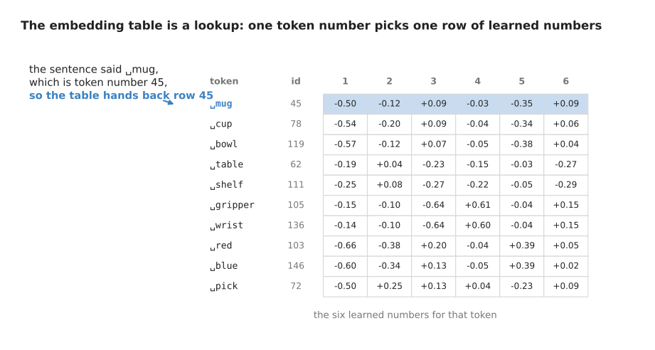
The full table has one row for each of the 429 tokens, and token number 45 picks out the shaded row.
The lookup is as simple as it sounds. The tokeniser says the word is token number 45. The model goes to row 45. It takes the six numbers that are there. The same token always gets the same row.
Those numbers start as small random values. Gradient descent then changes them, along with every other weight in the model. By the end of training they are whatever values made the model's predictions good. Libraries call this a layer rather than a lookup, and the next picture shows why.
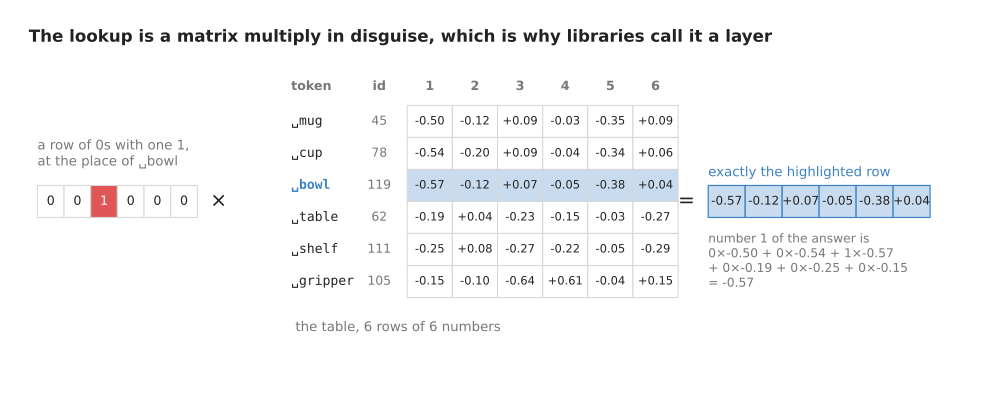
Picking row three is the same arithmetic as multiplying the table by a row of zeros that has a single one in the third place.
Write the token as a row of zeros with a single 1 at its own place, and multiply that row by the table. In every column, every term is zero except the one that is multiplied by 1. The answer is therefore exactly the chosen row. Column one is calculated as 0 times -0.50, plus 0 times -0.54, plus 1 times -0.57, plus three more terms that are all zero, which gives -0.57.
Nobody does this multiplication in practice, because reading row 45 out of memory is far cheaper. Writing the lookup this way is still useful, because it explains why the table is trained exactly like any other matrix of weights. The table is small on this page because the vocabulary is small. In a real model it is not small, as the next picture shows.
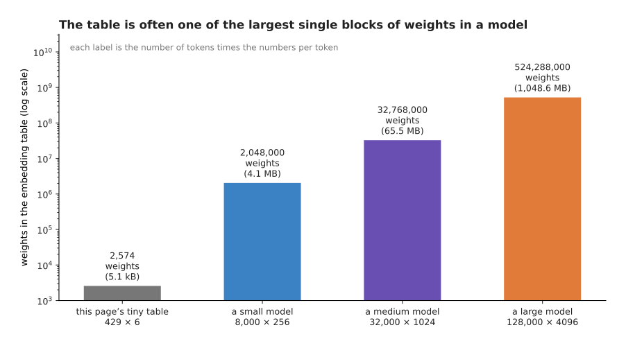
Each bar is one embedding table, and its label gives the weights it holds and the memory those weights need when each weight is stored in two bytes.
The table on this page holds 429 times 6 weights, which is 2,574. A small model with a vocabulary of 8,000 and 256 numbers a token holds 2,048,000 weights, which is 4.1 megabytes. A medium model with a vocabulary of 32,000 and 1,024 numbers a token holds 32,768,000 weights, which is 65.5 megabytes. A large model with a vocabulary of 128,000 and 4,096 numbers a token holds 524,288,000 weights, which is a little over a gigabyte. That last figure is often the single largest block of weights in a model.
The width of a row matters for a second reason. It is also the width that runs through every layer after the lookup, so it is chosen once and the rest of the model follows it. What makes those numbers useful is not their size but where they sit relative to each other, and the next section measures that.
4. Near each other means used in the same way#
Training never tells the table what any word means. The rows are still arranged in a way that is easy to describe. This section explains what that arrangement is, and how it is measured.
Two rows count as similar when they point in the same direction. The measure of that is called cosine similarity. To calculate it, multiply the two vectors number by number, add up the products, and divide the total by the length of each vector. A vector's length is the square root of the sum of its squares. The answer runs from +1, which means the two point in exactly the same direction, through 0, which means they are unrelated, down to -1, which means they point in exactly opposite directions.
The next picture does that calculation twice. Read each column downwards: the two rows are multiplied number by number, the six products are added, and the total is divided by the two lengths.
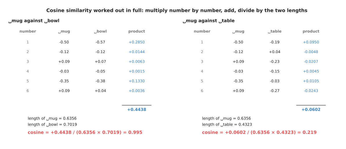
Cosine similarity is calculated in full twice, and it gives 0.995 for mug against bowl and 0.219 for mug against table.
For mug and bowl the six products add up to 0.4438. The two lengths are 0.6356 and 0.7019, and dividing gives 0.995. For mug and table the products add up to only 0.0602, and the same division gives 0.219. The arithmetic is identical both times. The difference lies entirely in the rows, and those rows came from counting which words appear near which other words in the invented instructions.
Doing that calculation for every pair of tokens gives a picture of the whole arrangement. In the picture below, each square is one pair, and a darker square means a higher score. The squares along the diagonal compare a token with itself, so they are all 1.00.
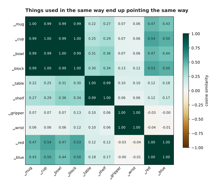
Every pair of ten tokens is scored, and four dark blocks appear where things are used in the same way.
Mug, cup, bowl and block score 0.99 or 1.00 against each other. Table and shelf score 0.99. Gripper and wrist score 1.00. Red and blue score 1.00. Mug against gripper scores only 0.07. Nobody labelled any of these words. The blocks appear only because words used in the same position in the same kinds of sentence have the same neighbours.
The obvious alternative to cosine similarity is straight-line distance between the ends of the two vectors, so it is worth saying why cosine is used instead.
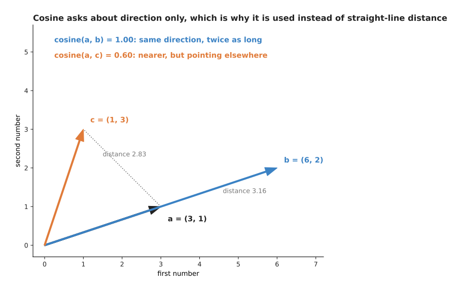
Arrow b points in exactly the same direction as a and scores 1.00, while arrow c is nearer in a straight line and scores only 0.60.
Arrow b is twice as long as a and points in exactly the same direction, so cosine gives 1.00 even though the distance between the two tips is 3.16. Arrow c ends only 2.83 away, and it scores 0.60, because it points somewhere else.
In an embedding table, the length of a row tends to follow how often that token appears, rather than what the token is used for. Throwing the length away and keeping only the direction is therefore what makes the measure say something about the token itself.
Asking which rows are nearest to a given row is the usual way to inspect a trained table. The next picture asks that question four times. Each small chart is one query token, and the bars are the five tokens nearest to it.
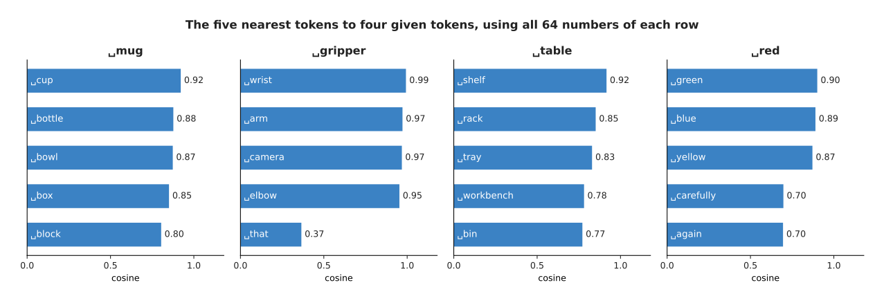
The five nearest tokens to each of four given tokens, found using all 64 numbers of a row rather than only the six that fit in a picture.
The tokens nearest to "mug" are cup at 0.92, bottle at 0.88, bowl at 0.87 and box at 0.85, and all of those are things an arm picks up. The tokens nearest to "gripper" are wrist at 0.99, arm at 0.97, camera at 0.97 and elbow at 0.95, and all of those are parts of the robot. After elbow the list falls to 0.37, because the text holds only four such words. The tokens nearest to "red" are green, blue and yellow, and then "carefully" at 0.70. That last one is a reminder that the grouping follows sentence position rather than meaning.
Everything in this section treats the tokens as an unordered collection. That is exactly the problem the next section fixes.
5. Telling the model what order the tokens came in#
Having a row for each token is not yet enough. The attention step that follows takes the tokens as a set. It compares every token with every other token, and it does not care which token came first. That claim is easy to show rather than simply assert.
The next picture takes two sentences made of the same six tokens in a different order, and adds up the six rows of each.
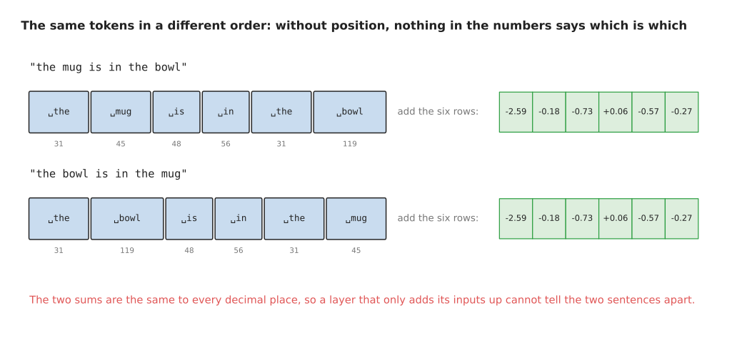
"The mug is in the bowl" and "the bowl is in the mug" are the same six tokens, so adding their rows gives exactly the same six numbers.
Both sentences become the tokens for "the", "mug", "is", "in", "the" and "bowl". Adding the six rows gives -2.59, -0.18, -0.73, +0.06, -0.57 and -0.27 in both cases, to every decimal place, because addition does not care about order. A robot told to put the mug in the bowl would therefore do the same thing as a robot told to put the bowl in the mug. The order has to be put into the numbers deliberately, and anything that does this is called a positional encoding.
The most direct method is to keep a second table. This table has one row for each place in the sentence, rather than one row for each token. It is learned during training, exactly like the first table. The row for the place is then added to the row for the token.
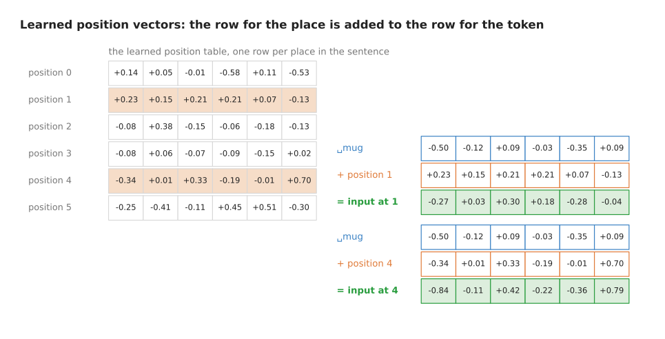
The same token at two different places in the sentence becomes two different lists of numbers, once the position row has been added.
The token for "mug" is -0.50, -0.12, +0.09, -0.03, -0.35, +0.09 wherever it appears. At position 1 it becomes -0.27, +0.03, +0.30, +0.18, -0.28, -0.04. At position 4 it becomes -0.84, -0.11, +0.42, -0.22, -0.36, +0.79. The cosine similarity between those two results is only 0.554, so the model can now tell the two apart.
This method costs two things. First, the table has a fixed number of rows, so a sentence longer than the table has places for cannot be handled at all. Second, the row for a late place is trained by very little text, because only long sentences reach that place. The next picture measures the second cost on this page's 3,200 instructions.
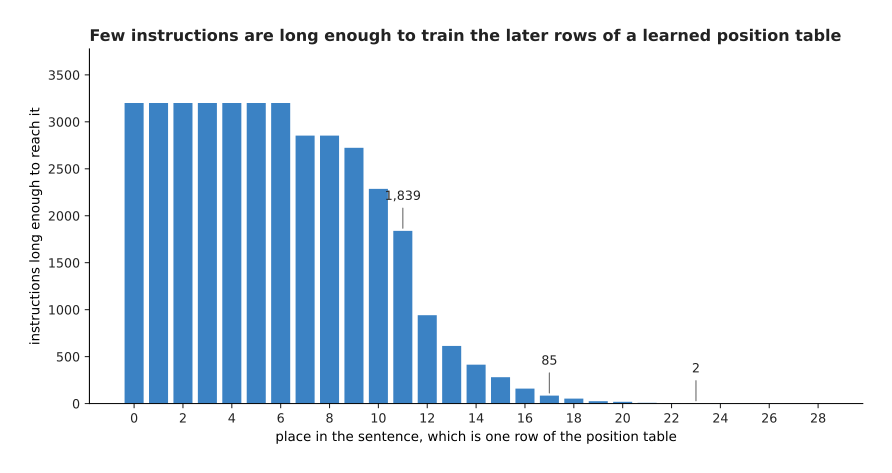
Every instruction trains the rows for the early places, and almost none of them trains the rows for the late places.
The 3,200 instructions are between 7 and 29 tokens long, and 11.74 tokens long on average. Places 0 to 6 are reached by all 3,200 of them. Place 11 is reached by 1,839 of them, which is 57.5 per cent. Place 17 is reached by 85 of them, which is 2.7 per cent. Place 23 is reached by 2 of them. A row that has been trained twice is not a trained row, so this method becomes unreliable exactly where sentences become long.
The method that almost every current model uses instead is called rotary position embedding, often shortened to RoPE. It turns the numbers instead of adding to them. The row is taken two numbers at a time. Each pair is treated as a point on a flat sheet. That point is then turned about the origin by an angle, and the angle grows in proportion to the place in the sentence. Each pair is given its own turning rate, so some pairs turn quickly and others barely move.
The next picture draws three pairs of the same token. Each circle is one pair, and the six arrows inside a circle are the six places 0 to 5.
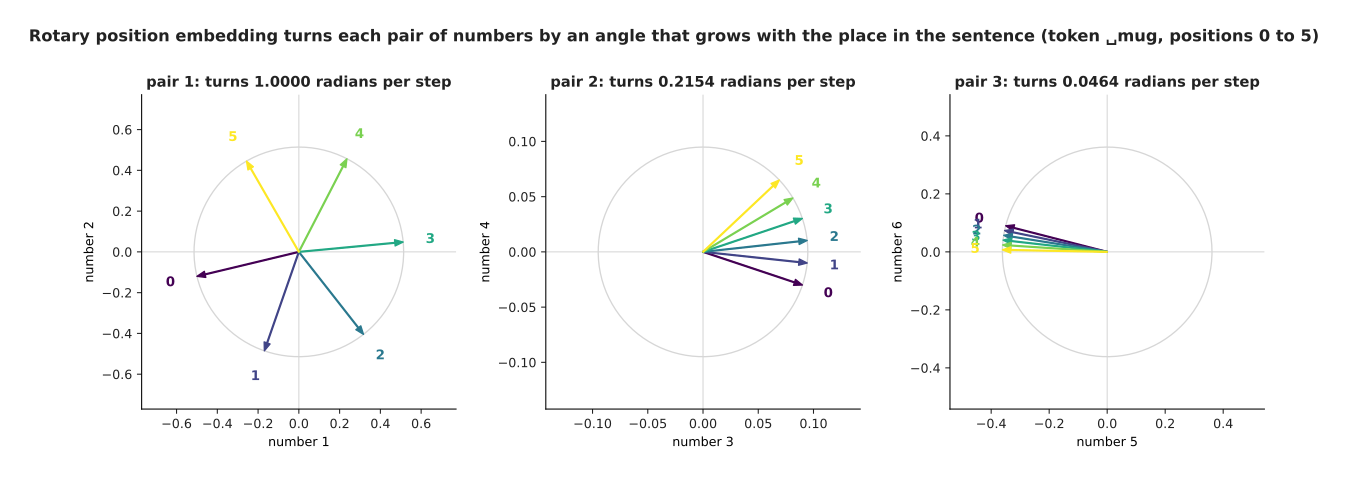
The same token is drawn at positions 0 to 5. Its first pair of numbers turns 1.0000 radians at each step, its second pair turns 0.2154 radians, and its third pair turns 0.0464 radians.
The first pair of the row for "mug" starts at (-0.500, -0.120) at position 0. By position 3 it has become (+0.512, +0.048), which is the same point turned three radians round the circle. The turning rates here were made large on purpose, so that the movement is visible over six positions. A real model uses far smaller rates, so its slowest pairs have barely turned even after thousands of positions.
Turning has one property that adding does not have. Turning a pair of numbers never changes how far that pair is from the origin, so the length of the whole row stays the same. The next picture measures that length at ten places, under both methods.
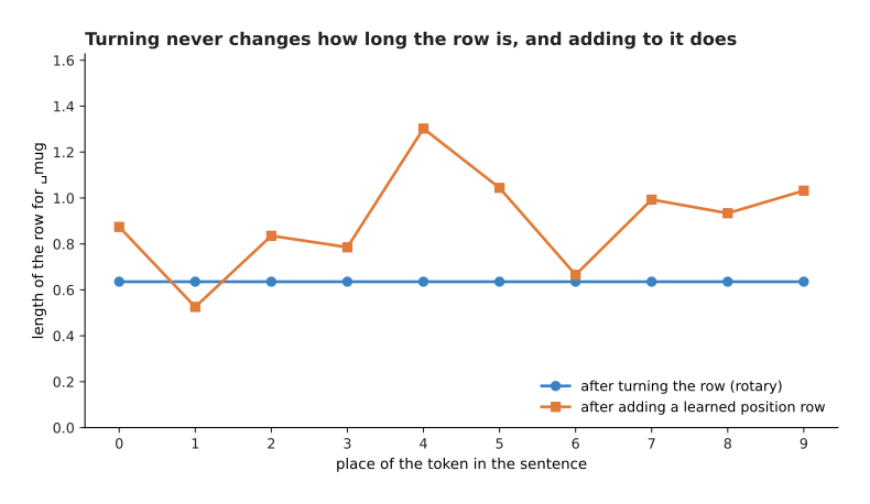
Turning leaves the length of the row exactly as it was, and adding a position row changes it at every place.
The row for "mug" is 0.6356 long. After turning it is 0.6356 long at every one of the ten places, to every decimal place the script prints. After a learned position row is added, the length moves between 0.5255 and 1.3024. A length that changes with the place means the size of the numbers entering the next layer changes with the place too, and keeping that size steady is one of the things that makes training behave, as Normalisation and stability explains.
The main reason to prefer turning over adding, however, is that it changes what attention measures. The next picture multiplies one turned row with another and adds the products, which is the arithmetic inside attention. Each row of the table is one pair of places with the same gap of three between them.
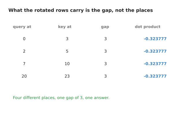
Four different pairs of places with the same gap give exactly the same answer, because turning both rows leaves only the difference between their two angles.
When one turned row is multiplied with another and the products are added, the two angles only ever appear as their difference. The answer therefore depends on how far apart the two tokens are, and not on where either of them sits. One row at place 0 multiplied with another row at place 3 gives -0.323777. Places 2 and 5 give the same. So do places 7 and 10, and places 20 and 23. Attention calls those two rows the query and the key, and Attention explains what each one is for. Without any turning the answer is +0.453112 whatever the gap, because nothing in the numbers mentions the places at all.
That property is what lets rotary position embedding work on sentences longer than anything seen in training. There is no table of positions that a long sentence can exceed, and a gap of three means the same thing at position 20,000 as it does at position 3. The cost is that the method only applies inside attention, on the query and key rows. It is therefore part of that step, rather than something you can do once at the input and then forget.
6. What the picture of the geometry leaves out#
Everything so far has described the table as a space with directions in it. That description is useful, and it is also drawn in a misleading way almost everywhere. This section says plainly what is true about it and what is not.
The first thing to be careful about is the flat scatter plot of words that appears in every talk on this subject. A scatter plot has two directions, and a row of this table has 64 numbers, so the plot has to choose two directions to look along and throw the rest away. The next picture makes that choice twice, with the same twelve rows.
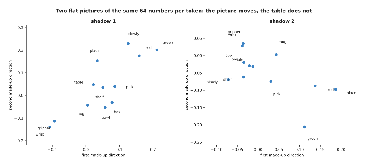
The same twelve rows of 64 numbers are flattened onto two different pairs of directions, so the picture changes completely while the table has not changed at all.
In the first plot the distance from mug to bowl is 0.053, and the distance from mug to gripper is 0.121, so mug looks much nearer to bowl. In the second plot those distances become 0.081 and 0.086, which are nearly equal. Neither plot is wrong, and neither is the truth. The arrangement is the 64 numbers, and the plot is only a choice of two directions to look along. In a real model each row holds a few thousand numbers, so the loss is greater still.
How much is lost in that flattening can be measured rather than guessed. The next picture plots every pair of tokens twice. The horizontal position of a dot is the real cosine similarity, using all 64 numbers. The vertical position is the cosine similarity after most of the numbers have been thrown away. A dot on the dashed line means the two agree.
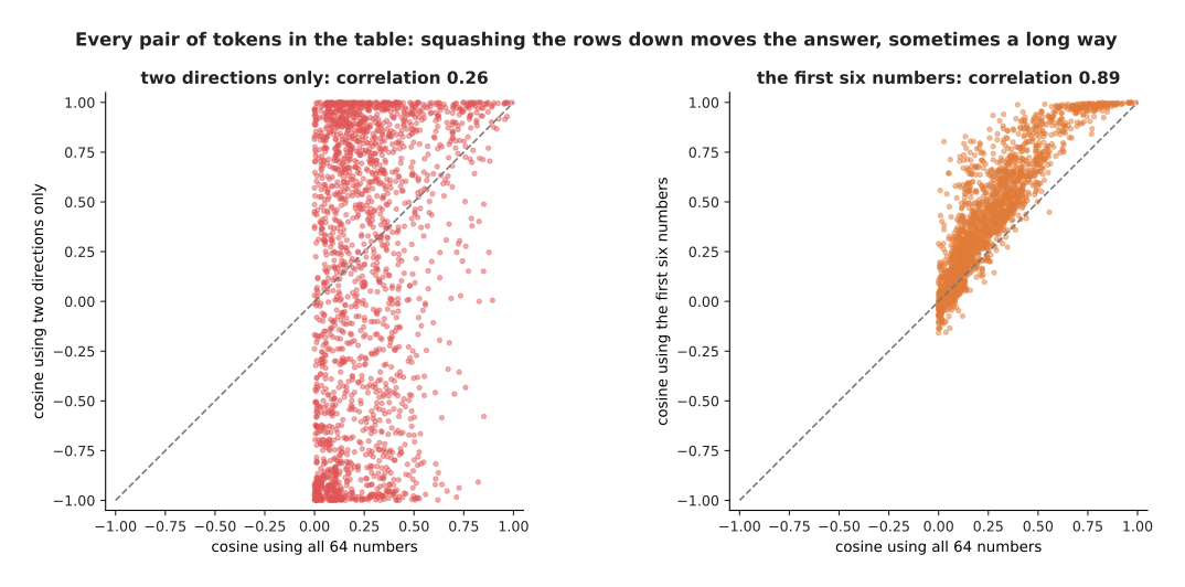
All 2,016 pairs of tokens in the table are drawn, which compares the real cosine with the cosine you get after throwing most of the numbers away.
Flattening to two directions and then measuring cosine tracks the real answer with a correlation of only 0.26, and the worst pair is wrong by 1.73. The scale runs from -1 to +1, so an error of 1.73 means the picture reverses the relationship completely. Keeping the first six numbers does better, with a correlation of 0.89, and even there the worst pair is wrong by 0.78. That is why section 4's scores for mug, cup and bowl were all 0.99 using six numbers, and spread out to 0.92 and 0.87 using all 64.
The second thing to be careful about is the idea that a row holds the meaning of a word.
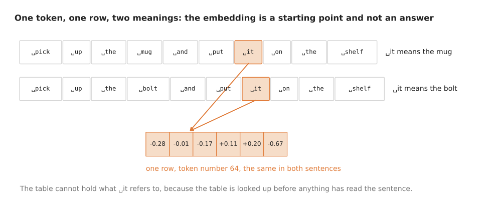
The token "it" has exactly one row in the table, and that row is the same whether "it" means the mug or the bolt.
The lookup happens before anything has read the sentence, so the table cannot possibly hold what "it" refers to. The same is true of every word that has more than one sense. What the row holds is a starting point that is good on average across all the uses of that token. The work of making it specific to this sentence is done afterwards, by the attention layers, which mix each token's numbers with the numbers of the tokens around it. By the middle of a trained model, the numbers where "it" sits are nothing like the row that was looked up. That is the intended behaviour and not a fault.
The third thing to be careful about is the idea that each direction in the table stands for one property. There are far more properties worth representing than there are numbers in a row, so several properties have to share each direction. That sharing is possible because directions do not have to be exactly separate to be useful, and the next picture measures how much sharing 64 numbers allow.
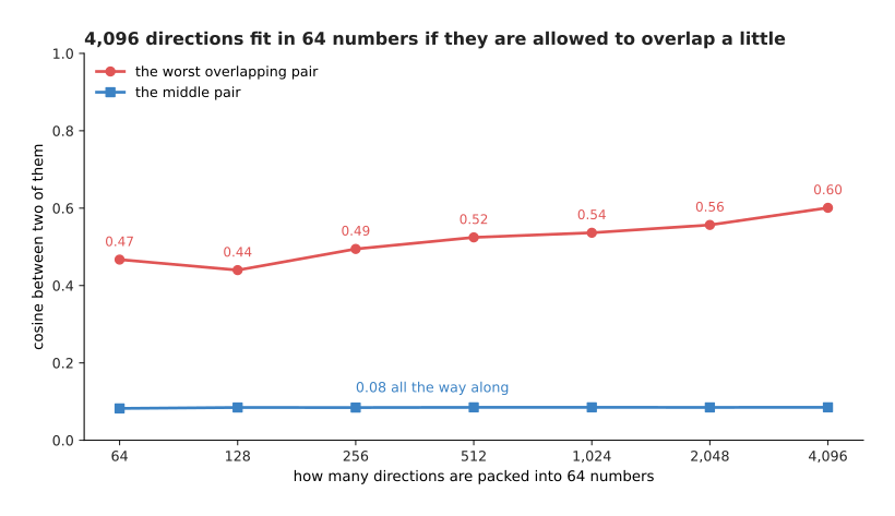
Thousands of directions fit into 64 numbers, as long as they are allowed to overlap a little.
Only 64 directions can be exactly separate in 64 numbers, which means a cosine of 0 between every pair. If a small overlap is allowed, far more fit. With 4,096 random directions packed into 64 numbers, the middle pair still has a cosine of 0.08, and even the worst pair has a cosine of 0.60. As the count rises from 64 directions to 4,096, the middle pair does not move at all, and the worst pair stays between 0.44 and 0.60.
Because properties share directions this way, a single direction read off a trained model usually turns out to mean several things at once. The next picture takes one direction of this page's table and lists the tokens that reach furthest along it in each sense.
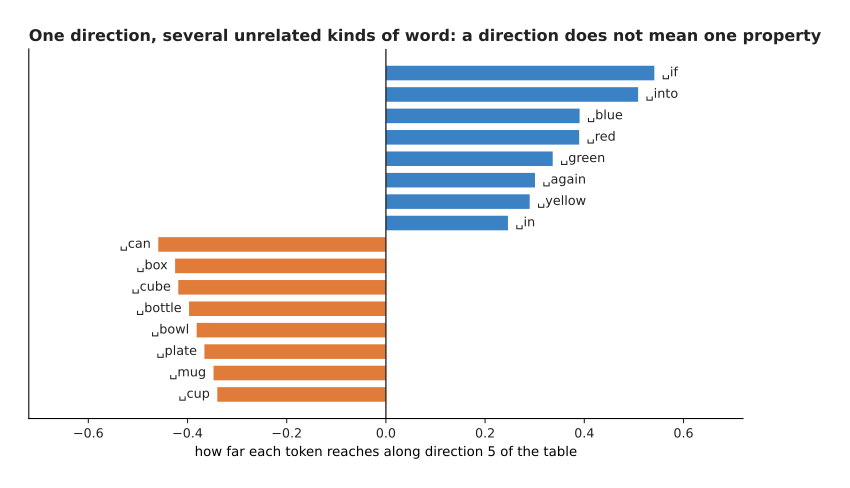
One direction of the table mixes grammar words with colour words at one end, and holds containers at the other end.
At the positive end of this direction sit "if" at +0.54, "into" at +0.51, "blue" at +0.39, "red" at +0.39, "green" at +0.34 and "again" at +0.30. Those are not one kind of word. At the negative end sit "can" at -0.46, "box" at -0.42, "cube" at -0.42 and "bottle" at -0.40, which are containers. So this one direction is carrying at least two unrelated distinctions, and reading it as "the colour direction" would be wrong.
The honest summary is this. The table is a learned convenience. It puts tokens that are used alike in similar places, which is genuinely useful. The flat pictures people draw of it are shadows of something that nobody can see directly.
7. Where to read next#
- Pictures, sound and robot states is the next page, and it does this same job for photos, depth pictures, point clouds, sound and the arm's own readings.
- Attention is where these tokens are actually used, and where section 5's rotary position embedding is applied.
- A transformer block shows how a stack of such blocks turns the looked-up rows into something that depends on the sentence.
- Training and running a transformer explains next-token prediction, the job that gives the table its numbers.
- Language models is the catalogue of real language models used on robot arms.
- Vision-language models covers models that read a picture and a sentence together, which need both this page and the next one.
8. Using it in Python#
Section 1 cut a sentence into eleven tokens. Section 3 looked those tokens up in a table of 429 rows of 6 numbers. Section 4 measured two rows against each other. Section 5 turned a pair of numbers by an angle. The code below does all four, on the exact numbers this page printed, so you can check every value against the pictures above.
import torch
from torch import nn

# Section 3: the embedding table, as a layer. 429 tokens, 6 numbers each.
table = nn.Embedding(num_embeddings=429, embedding_dim=6)
print(table.weight.shape)                           # torch.Size([429, 6])
print(sum(p.numel() for p in table.parameters()))   # 2574

# Section 1: the tokeniser has already turned the sentence into these numbers.
ids = torch.tensor([[72, 73, 31, 146, 45, 51, 69, 64, 38, 31, 121]])
print(table(ids).shape)                             # torch.Size([1, 11, 6])

# Section 4: cosine similarity, on the rows printed in section 3.
mug   = torch.tensor([-0.50, -0.12,  0.09, -0.03, -0.35,  0.09])
bowl  = torch.tensor([-0.57, -0.12,  0.07, -0.05, -0.38,  0.04])
table_row = torch.tensor([-0.19,  0.04, -0.23, -0.15, -0.03, -0.27])
print(torch.cosine_similarity(mug, bowl,      dim=0))   # tensor(0.9947)
print(torch.cosine_similarity(mug, table_row, dim=0))   # tensor(0.2191)

# Section 5: rotary position embedding, on the first pair of numbers.
def turn(pair, place, rate):
    angle = place * rate
    c, s = torch.cos(angle), torch.sin(angle)
    return torch.stack([pair[0] * c - pair[1] * s, pair[0] * s + pair[1] * c])

pair = mug[:2]
print(turn(pair, torch.tensor(0.0), torch.tensor(1.0)))  # tensor([-0.5000, -0.1200])
print(turn(pair, torch.tensor(3.0), torch.tensor(1.0)))  # tensor([0.5119, 0.0482])
The library gives you the table, its random starting values, its gradients, and a lookup that handles a whole batch of sentences at once. It does not give you the tokeniser, because a tokeniser belongs to one particular model. The vocabulary, the merge list and the numbering were all fixed when that model was trained. Pairing a trained model with a different tokeniser therefore gives nonsense, because row 45 would then stand for a different piece of text.
In practice you load the tokeniser that came with the model. In Hugging Face's
transformers package that is AutoTokenizer.from_pretrained(name). You then
call it on your text to get the numbers that go into ids above.
That one choice settles most of the other decisions. A pretrained model fixes the vocabulary size, the width of a row and the kind of positional encoding, and changing any of them means training from the beginning again. The decision that stays yours is what text you put into the tokeniser. Text that is unlike anything the tokeniser was built from is cut into far more tokens than you expect, and those extra tokens cost time and context on every call. It is therefore worth measuring the token count of the text your robot will really produce, rather than assuming it matches the count of words.