Every page after this one uses the same handful of words, and uses them as though you already know them: supervised, self-supervised, reinforcement, machine learning, deep learning, foundation model. This page is where they get defined.
It is a reference page, not an argument. Each word is defined in one sentence, then shown doing its job on the cup task that this chapter has used throughout, so that you can see what the word refers to rather than only what it means. The last section walks that one task from start to finish and names every term in order, so if you only read one part of this page, read that one.
It is for a reader who has read what a model is, which already defined model, parameter, weight, training, inference, dataset, feature, label and generalisation. This page adds the words that chapter did not need.
Contents#
- Three ways a model is told what is right
- Artificial intelligence, machine learning, deep learning and foundation models
- Every word on one job from start to finish
- Where to read next
- Using it in Python
1. Three ways a model is told what is right#
The pages before this one assumed that somebody had written the right answer beside every example. That is only one of the three arrangements in use. The three differ in who supplies the right answer, not in the arithmetic, and all three are called learning.
Supervised learning is the arrangement used in the last two sections. Every example carries a label, and a person or an instrument wrote that label down. It gives the clearest training signal of the three, and its cost is the labelling. The chart below turns that cost into hours of a person's time, on a log scale.
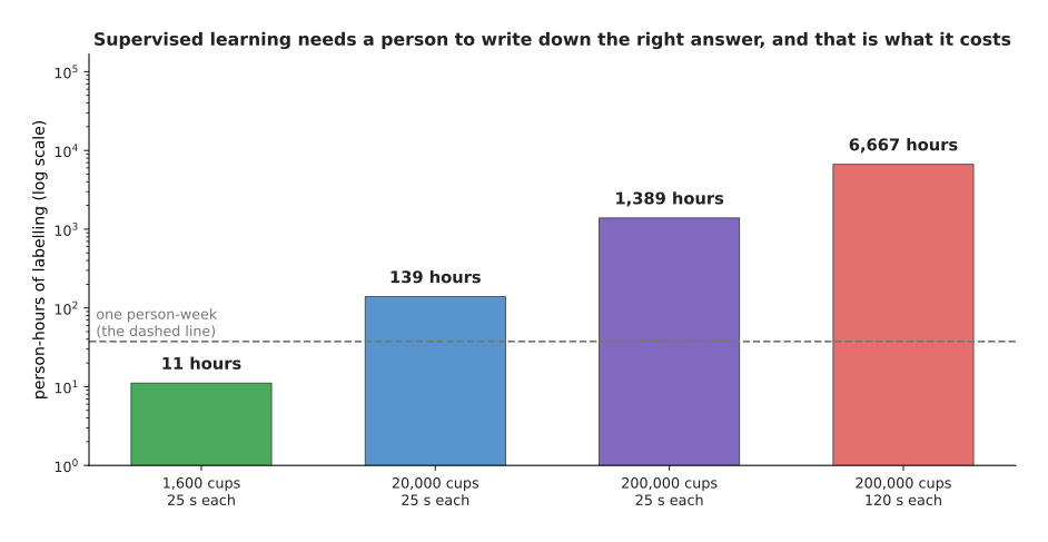
At 25 seconds a cup, labelling 1,600 cups takes 11 person-hours, 20,000 cups takes 139 and 200,000 cups takes 1,389. Some labels take much longer than 25 seconds. A careful outline drawn round an object takes about 120 seconds, and at that rate 200,000 examples take 6,667 person-hours.
Those hours are the reason why the next arrangement exists. Self-supervised learning hides part of the data and asks the model to produce the hidden part. So the data supplies its own answers, and nobody writes a label at all. The picture below does that with a recording of one joint angle.
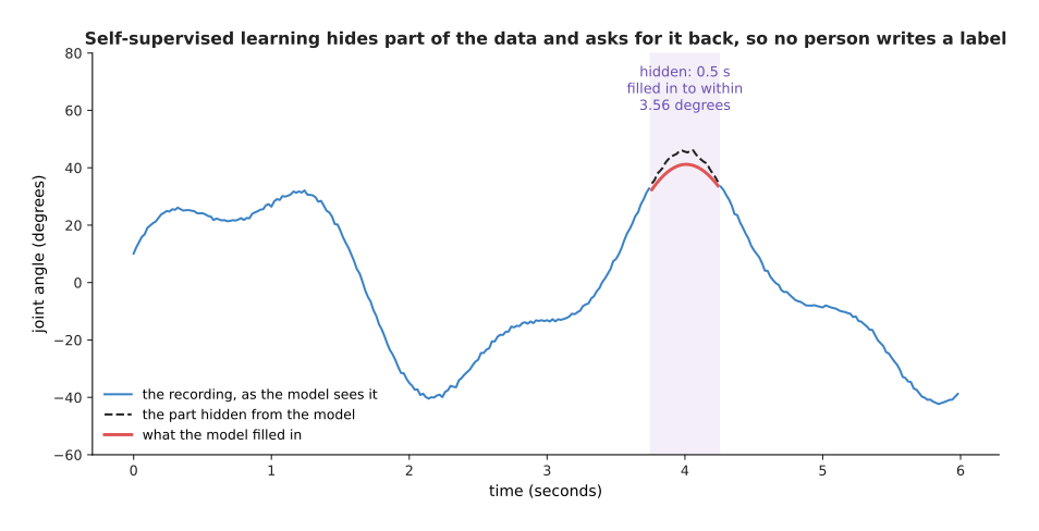
The recording holds 300 samples, and 25 of them were hidden, which is half a second. The hidden stretch includes the moment when the joint stops and turns the other way, so it is the hardest part to guess. Filling it in from the samples on each side gives an answer that is out by 3.56 degrees on average and by 5.26 degrees at worst.
Nobody labelled the gap in that picture. The recording already contained the answer, and the answer was simply covered up. This matters far more than it looks, because it means that a model can be trained on data that nobody has annotated, which is almost all the data there is. Self-supervised pretraining shows that nearly every large model in use today was trained this way.
The third arrangement has no answers at all, only outcomes. Reinforcement learning lets the model try something, scores whether the attempt worked, and uses that score to change what it tries next. The picture below shows 400 simulated attempts at a grasp, in blocks of twenty, and how often the attempts in each block worked.
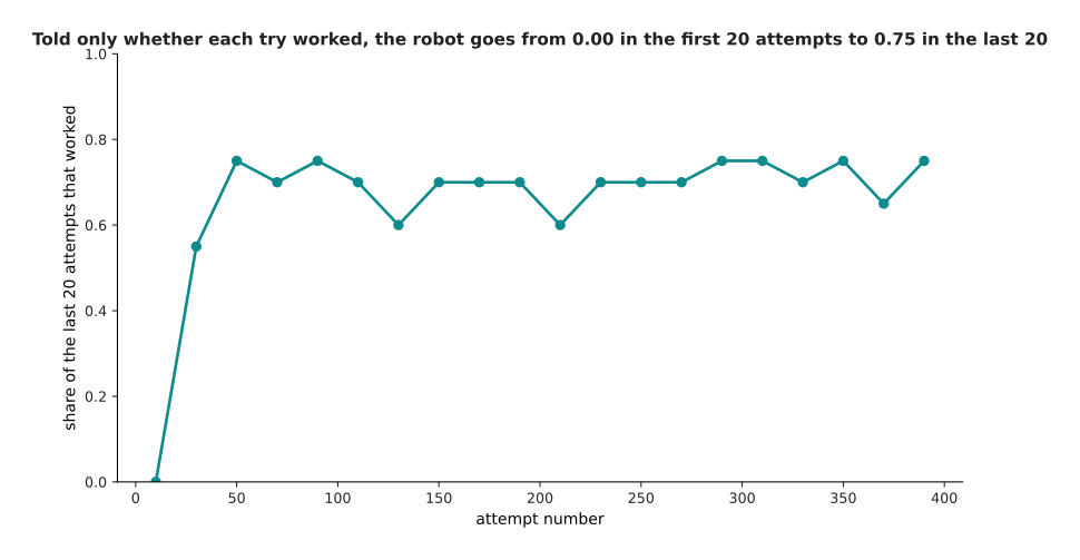
The share of attempts that worked rises from 0.00 in the first twenty attempts to 0.75 in the last twenty. Of the 400 attempts, 264 succeeded. The picture below shows the same 400 attempts one at a time, with the height that each attempt tried up the page, and the colour saying whether that attempt lifted the object.
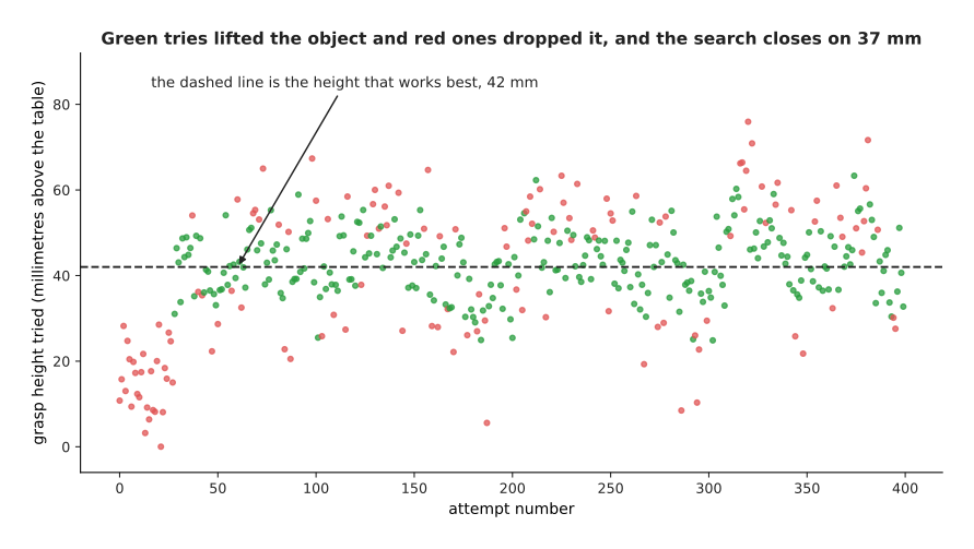
The best height for this simulated grasp is 42 millimetres above the table. The search starts far below that, near 18 millimetres. Each time an attempt works, the search moves its preferred height towards the height that just worked, and then it tries again near the new preferred height. After 400 attempts it has settled on 37.4 millimetres.
Nobody ever told that search what the right height was. It found 37.4 millimetres from nothing except 400 answers of the form "that worked" or "that did not work". The cost is inside that sentence, because the 136 failures were real attempts on a real arm, with a real object falling on the floor. Reinforcement learning goes through how the scores turn into better attempts, and why most of this happens in simulation.
The three arrangements are easiest to compare by what a person has to supply. The chart below counts exactly that, on a log scale, for the three ways above.
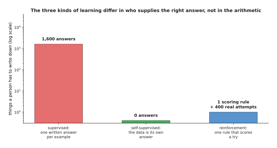
For the cup job, supervised learning needs 1,600 written answers. Self-supervised learning needs none, because the hidden samples are the answer. Reinforcement learning needs one written scoring rule, plus 400 attempts on the real arm.
Read that chart with care, because the shortest bar is not the cheapest method. Writing the scoring rule for reinforcement learning is one line of work, and getting that one line slightly wrong produces a robot that scores well while doing something useless. The page rewards, preferences and verifiers is entirely about that problem. Self-supervised learning needs no labels, and in exchange it needs enormous amounts of unlabelled data. The three are usually combined rather than chosen between. The next section places all three inside the four names that people give to this field as a whole.
2. Artificial intelligence, machine learning, deep learning and foundation models#
The last four sections used four more words without defining them. They are the four words that people outside the field use as if they meant the same thing. They do not mean the same thing, because each one sits inside the one before it, as the picture below shows.
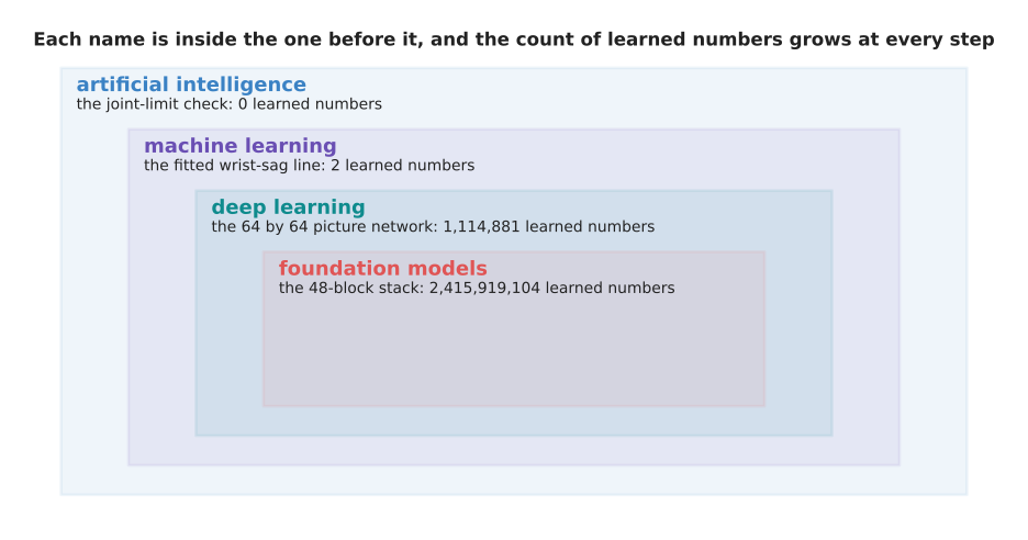
The joint-limit check named in how rules do the work sits in the outer rectangle and has 0 learned numbers. The fitted sag line sits in the second and has 2. The picture network sits in the third and has 1,114,881. A 48-block stack sits in the innermost and has 2,415,919,104.
Artificial intelligence is the outer rectangle. It is any program that does a job which people would call clever. The joint-limit check is inside it, which shows how wide the term is. The term is wide because it was named after the goal rather than after any method. It appears in every headline and it carries almost no information, so this book uses it as little as possible.
Machine learning is the second rectangle. It is the part of artificial intelligence where the program finds the numbers inside itself from examples, instead of being told them. Everything in this chapter so far, from the six measurements onwards, is machine learning, and so is the fitted line with its two parameters. The boundary is exactly the one drawn on that page, between a rule that somebody wrote and a formula that somebody fitted.
Deep learning is the third rectangle. It is the part of machine learning where the model is made of many layers of neurons stacked on top of each other, so that the output of one layer is the input of the next. The word deep means that there are many such layers, and it means nothing more than that. The picture below shows what those extra layers buy on one simulated job. Each point is a network of the same width, with a different number of layers.
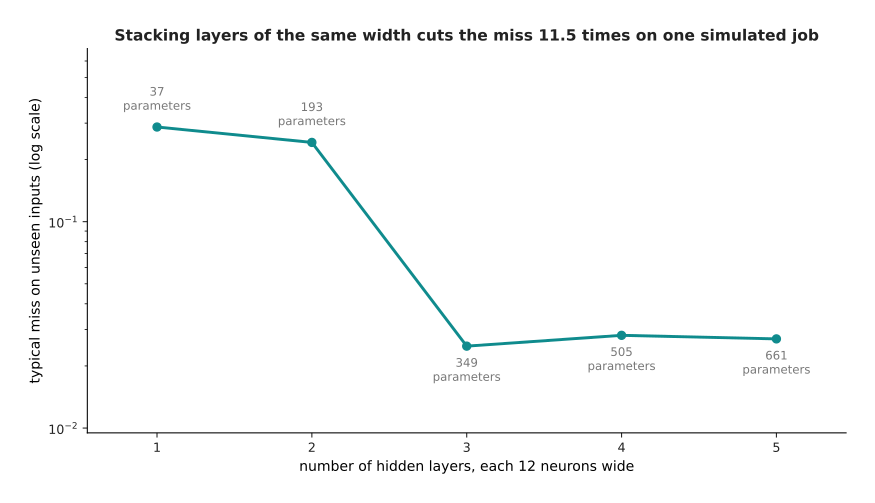
On this job, networks of 1 to 5 hidden layers of 12 neurons miss unseen inputs by 0.2873, 0.2420, 0.0249, 0.0281 and 0.0270. So three layers is 11.5 times better than one layer, and it reaches that while holding 349 parameters against 37.
The picture below shows what those numbers mean. It draws the shape that the networks were asked to match, and the shape that two of them actually produced.
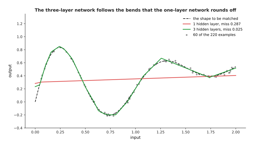
The one-layer network rounds off every bend in the target and ends up almost straight. The three-layer network follows the bends. What a network can learn explains why stacking layers has that effect, and layers and depth explains what a layer is. Almost every model that this book describes after chapter 2 is a deep model, which is why deep learning and machine learning are so often confused with each other.
A foundation model is the innermost rectangle. It is one large deep model, trained once on a huge and mixed pile of data, and then adapted to many different jobs instead of being built for one. The reason why anybody pays to train a model with billions of parameters is that the cost is shared between those jobs. The chart below shows the shared part beside the extra parameters that three different jobs need, on a log scale.
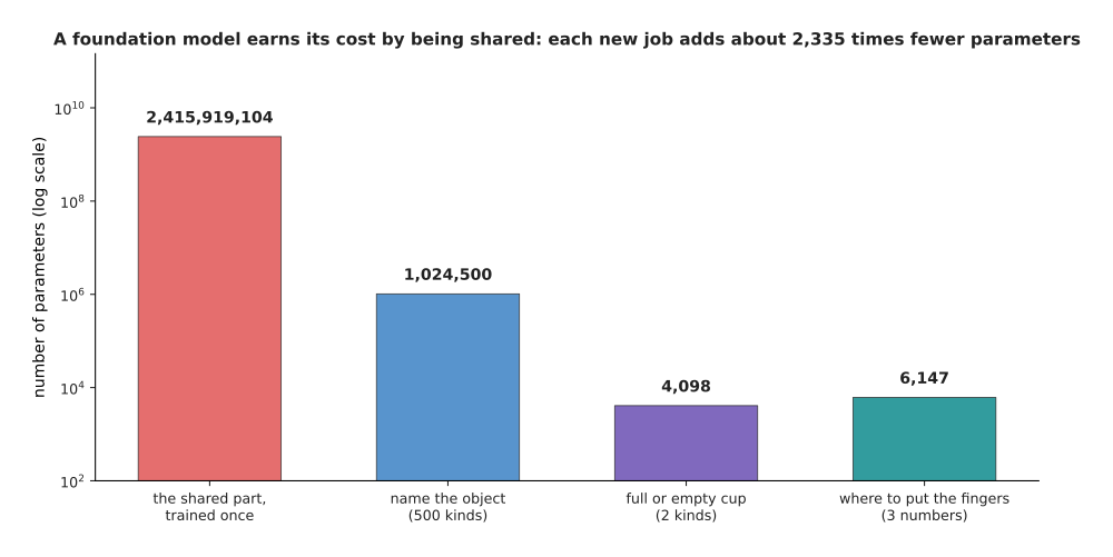
A shared 48-block stack holds 2,415,919,104 parameters. Adding a job that names one of 500 objects costs 1,024,500 more parameters. Adding a job that tells a full cup from an empty one costs 4,098, and adding a job that gives three finger positions costs 6,147. All three of those together are 2,335 times smaller than the shared part.
So the nesting is this. Every foundation model is a deep model. Every deep model is a machine learning model. Every machine learning model is artificial intelligence. None of those statements is true in the other direction. Fine-tuning and adapters is the page about how a job is actually added to a shared model. All four names now have a place, so the last section puts every word on this page onto one job at once.
3. Every word on one job from start to finish#
The cup job has appeared in every section above. This section runs through it once from end to end and names each word as it arrives, so that the vocabulary forms one connected story instead of a list. The picture below is the whole job in four boxes, filled with that job's real numbers. Read it from left to right.
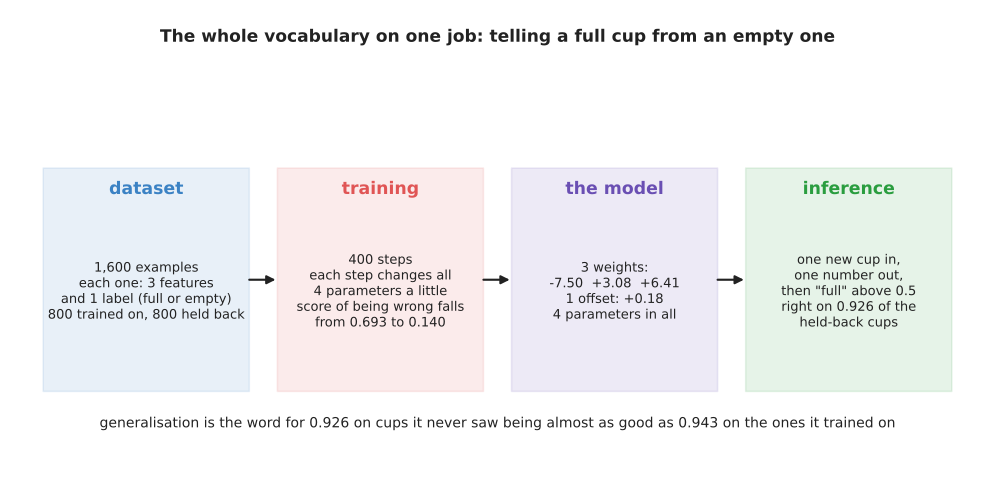
The dataset holds 1,600 examples, each with 3 features and 1 label, split into 800 for training and 800 held back. Training runs 400 steps and drops the score of being wrong from 0.693 to 0.140. The model is 3 weights and 1 offset. Inference turns one new cup into one number, and it is right on 0.926 of the held-back cups.
Here is the same thing in words. Somebody photographs 1,600 cups and writes beside each photograph whether that cup is full. That makes 1,600 examples, and therefore a dataset, and because a person wrote those answers it is supervised learning. Three numbers are measured from each photograph, and those three numbers are the features. Half of the examples are set aside and never shown to the training, so that the score on them at the end is a measurement of generalisation. The model is chosen to be three weights and one offset, which makes four parameters, and all four start at zero. Training then runs 400 steps, and each step changes all four parameters a little.
The picture below is that training run. The score of being wrong is on the vertical axis, and the step number is on the horizontal axis.
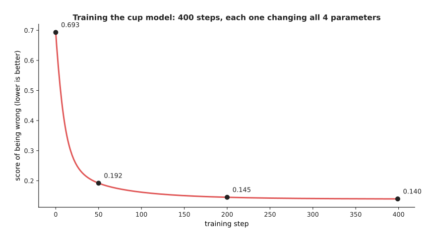
The score of being wrong is 0.693 at step 0, 0.192 at step 50, 0.145 at step 200 and 0.140 at the end. Training then stops, and the four numbers are finished.
After that, every held-back cup is put through the model once, which is inference happening 800 times. Each cup goes in as three numbers and one number comes out. The model calls the cup full when that number is above 0.5. The picture below counts the 800 answers.
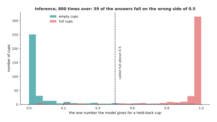
Most of the empty cups sit near 0 and most of the full cups sit near 1. The cups in the middle are the hard ones. In total, 59 of the 800 answers fall on the wrong side of 0.5, which leaves the model right on 0.926 of them.
The last thing to see is what separates training from inference. The difference is simply whether the four numbers are allowed to move. The picture below plots all four of them against the training step, and then carries them on into the shaded region, which is the time after training.
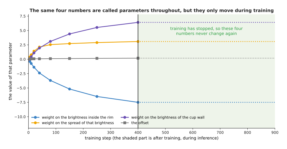
The three weights move from -0.080, +0.080 and -0.080 after one step to -7.497, +3.081 and +6.414 after 400 steps. The offset moves from +0.080 to +0.183. After that they never change again.
They are called parameters throughout, during training and afterwards. The only difference is that training moves them and inference does not. Everything that follows in this book is this same picture with more parameters in it. The next chapter opens the model box and shows what is inside when the formula is not a straight line but a network, starting with one neuron worked out by hand.
4. Where to read next#
One neuron opens a model up and works out by hand what the smallest piece inside it does. It is the next page of the book, and everything from here on is built out of that piece.
How training works explains how the search for good parameters actually proceeds, which this chapter has so far described only as "fitting".
5. Using it in Python#
The cup model used all through this chapter is small enough to build in one screen of NumPy, which is the array library that most Python numerical work is built on. The code below makes the same 1,600 simulated cups, fits four parameters to half of them, and scores itself on the other half. The comments name the idea each line belongs to.
import numpy as np

rng = np.random.default_rng(31)                                 # section 3: the dataset
n = 1600
full = rng.integers(0, 2, n).astype(float)                      # the label of each example
base = rng.uniform(90, 180, n) * rng.uniform(0.8, 1.2, n)       # cup colour times lighting
inside = base + np.where(full > 0.5, -18.0, 4.0) + rng.normal(0, 8, n)   # feature 1
spread = np.where(full > 0.5, 9.0, 4.0) + rng.normal(0, 2.2, n)          # feature 2
wall = base + rng.normal(0, 6, n)                                       # feature 3

X = np.column_stack([inside, spread, wall, np.ones(n)])   # section 1: 3 weights + 1 offset
train, test = slice(0, 800), slice(800, 1600)             # section 3: the split

w, *_ = np.linalg.lstsq(X[train], full[train], rcond=None)   # section 2: training
print(np.round(w, 4))                  # [-0.0166  0.0704  0.0159  0.0476]
print(X.shape, w.size)                 # (1600, 4) 4

seen = float(((X[train] @ w > 0.5) == (full[train] > 0.5)).mean())
unseen = float(((X[test] @ w > 0.5) == (full[test] > 0.5)).mean())
print(round(seen, 3), round(unseen, 3))   # 0.941 0.93    section 3: generalisation

one = X[test][0]                                             # section 2: inference
print(round(float(one @ w), 3), bool(one @ w > 0.5))         # 0.776 True
The library does two things here. First, it gives you arrays, so that
X[train] @ w works out all 800 answers in one expression rather than in a loop.
Second, it gives you np.linalg.lstsq, which finds the four parameters that make
the total squared miss as small as possible. That one call replaces the whole
training run of section 2, and it is exact rather than step by step. That is
possible only because this model is a weighted sum of its inputs. Every model later
in this book needs the step-by-step search instead, and for those the library you
reach for is PyTorch, where the same four parameters would be an nn.Linear(3, 1)
layer.
What the library will not decide is the shape of the problem. You choose the three
features. You choose to put a column of ones into X, so that the model has an
offset. You choose where to split the dataset. You choose 0.5 as the point above
which a cup is called full. Moving that last number trades one kind of mistake for
the other, because a lower threshold calls more cups full, so it catches more of
the full cups and it also calls some empty ones full by mistake.
Notice also that the printed scores are 0.941 on the half that was trained on and 0.930 on the half that was not. Those are the two numbers that section 3 said must always be reported together. The exact fit here and the step-by-step fit used for the diagrams reach slightly different parameters and nearly the same scores. That is the ordinary situation rather than a problem. Two training methods that reach the same quality of answer are both correct, and you pick between them on cost rather than on the answer.