The page before this one, reasoning and tool use, ended a long run of pages about models that are trained by being shown the right answer. In every one of those methods, a person had to write the right answer down first. This page is about the opposite situation. Sometimes nobody knows the right answer in advance, but anybody can look at what happened afterwards and say whether it went well.
That situation is common on a robot arm. Nobody can write down the joint angles that pick up a particular mug, because the correct angles depend on where the mug stands and on how the fingers touch it. After the attempt, however, it is easy to say whether the mug is in the gripper. Reinforcement learning is learning from that kind of judgement, made after the event rather than before it. The learner tries something. Then one number comes back that says how good the result was. Over many tries the learner changes what it does, so that the number becomes larger.
This page explains the parts of that idea on one small example. After that it explains the three things that make reinforcement learning hard. The first is that the learner has to try actions it does not believe in. The second is that each improvement has to be small, so that it does not destroy the behaviour that already works. The third is that the number of tries needed is far larger than a real arm can survive. By the end you will know the words that every text on this subject uses, you will have seen a policy learned from nothing at all, and you will know why this work is almost always done in a simulator. The page assumes you have read gradient descent and the words everyone uses.
The world in every picture is invented rather than measured from a real arm, and
the program docs/diagrams/learning_from_outcomes.py works out every number
shown. The learning is real. The policies are learned from nothing by tabular
Q-learning and by a clipped policy-gradient step, both written in NumPy, and both
are checked against exact answers from value iteration.
Contents#
- The pieces: state, action, reward, episode and return
- The policy and the value function
- Learning the whole thing from nothing
- Exploring against taking the best answer you know
- Whose attempts you learn from, and how big a step to take
- Why this happens in a simulator, and what the crossing costs
- Where to read next
- Using it in Python
1. The pieces: state, action, reward, episode and return#
Reinforcement learning has no right answers to copy, so it needs a different set of words from the rest of this book. This section introduces those words on one example that is small enough to draw in full.
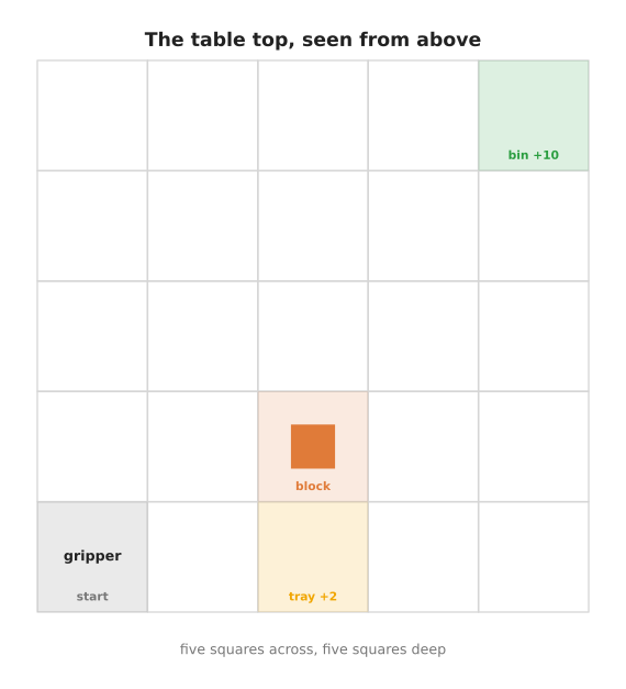
The example is a table top of five squares by five. A gripper stands on the table and moves one square at a time. One block lies on the table. A bin stands in the far corner, and the block should be placed in that bin. A tray stands near the block, and somebody has decided that the tray also counts as a place to put things. The picture below shows the four squares that matter.
The gripper can do seven different things, and the table below lists all of them. Read the first column as the name of the action, the second column as the reward that arrives immediately after it, and the third column as what the action changes in the world. Every action costs a little, so a gripper that does nothing useful loses reward.
| action | reward | what it does |
|---|---|---|
| up, down, left, right | −0.10 | move one square; a wall leaves the gripper where it was |
| close | −0.15 | shut the fingers; this picks the block up if the gripper stands on it |
| open | −0.15 | let go; the bin then pays 10, the tray pays 2, and any other square costs 1 more because the block falls |
| wait | −0.10 | hold the pose and change nothing |
The attempt stops as soon as the block is put down on the bin or on the tray. It also stops after 80 actions, whichever happens first.
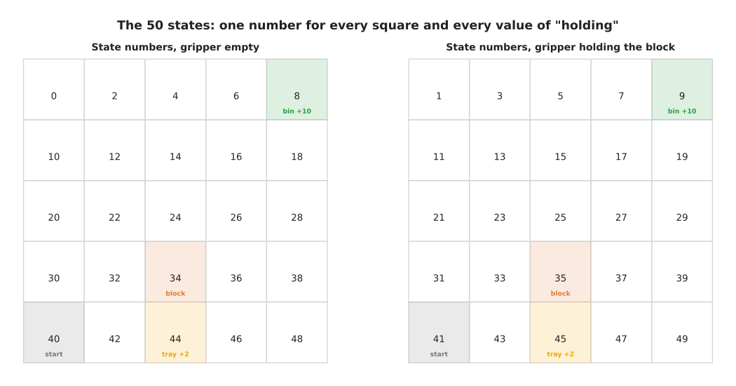
The first word is the state. The state is everything the learner can see at one moment. In this example the state is the square the gripper stands on, together with whether the gripper holds the block. There are 25 squares and two values of "holding", so there are 50 states in all. On a real arm the state is the joint angles, the gripper opening and a camera picture instead.
Each of those 50 states is given a number, so that the learner can use the number as an index into a table. The next picture shows every state number. The two halves of the picture show the same 25 squares, once for an empty gripper and once while the block is held.
The second word is the action. An action is one of the things the learner can choose to do. Here there are seven actions, which are the four moves, closing the gripper, opening it, and waiting. Choosing an action changes the state, and the picture below shows what each of the seven actions does from one particular state. That state is number 34, which means the gripper stands on the block's square with nothing in its fingers.
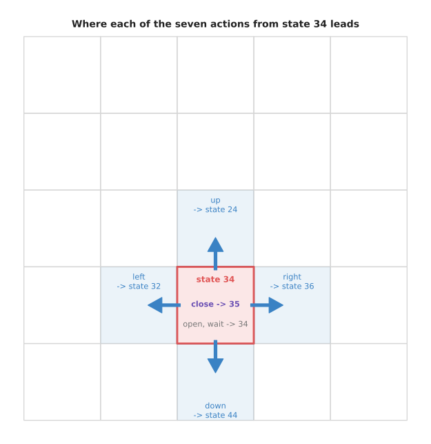
Closing the gripper on the block moves the learner from state 34 to state 35, because 34 and 35 are the same square with a different value of "holding".
The third word is the reward. A reward is a single number that arrives after each action and says how good the result was. A reward is not advice, because it never says what should have been done instead. That is what makes this different from the earlier chapters of this book, where every example came with its correct answer attached. In this world every action costs 0.10, a gripper command costs another 0.05, and the bin pays 10. The action that finishes the job is therefore worth 10 minus 0.15, which is 9.85.
The next picture shows one whole attempt. The left side draws the route the gripper took, and the right side draws the reward that came back after each of its ten actions. Both sides describe the same attempt.
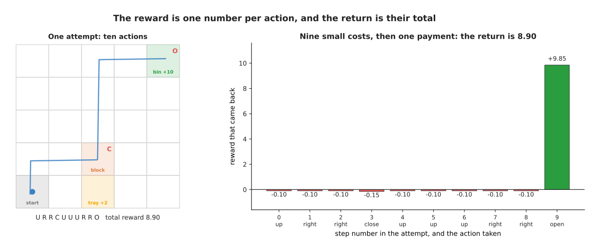
The best attempt takes ten actions. Nine of them cost a little and one pays 9.85, so the whole attempt collects 8.90.
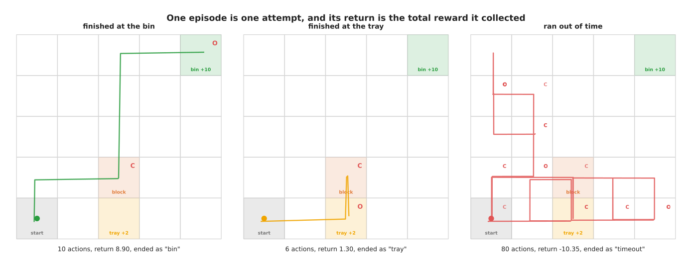
The fourth word is the episode. An episode is one whole attempt. An episode ends here when the block is put down, or when 80 actions have been used. The fifth word is the return. The return of an episode is the total of all the rewards collected during it. The picture below shows three real attempts and the return of each.
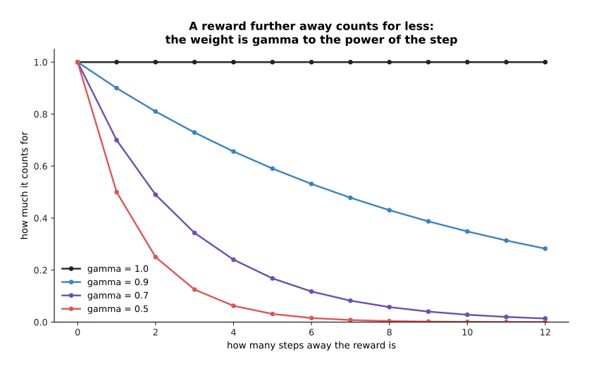
One more piece of the idea is less obvious. A reward that arrives later usually counts for less than the same reward arriving now. How much less is set by the discount factor, which is written as the Greek letter gamma. A reward one step away is multiplied by gamma. A reward two steps away is multiplied by gamma twice, and so on. The total worked out in that way is called the discounted return. The picture below shows the weight itself for four values of gamma.
There are two reasons for discounting. The first is that a robot which finishes sooner is worth more than one which finishes later. The second is that without the weight the sums in section 2 would grow without limit. The next picture applies the weight to the ten rewards of the attempt above, so you can see what it does to a real route.
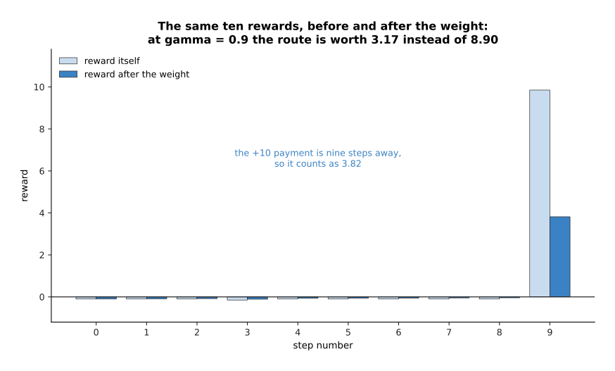
The payment at the bin is nine steps away from the start of the attempt, so at a gamma of 0.9 it counts as 3.82 rather than 9.85. The whole route is then worth 3.17 rather than 8.90.
Discounting does more than make the numbers smaller. It can change which behaviour is best. The bin pays five times what the tray pays, but the route to the bin is four actions longer than the route to the tray. The picture below compares the two routes at four values of gamma.
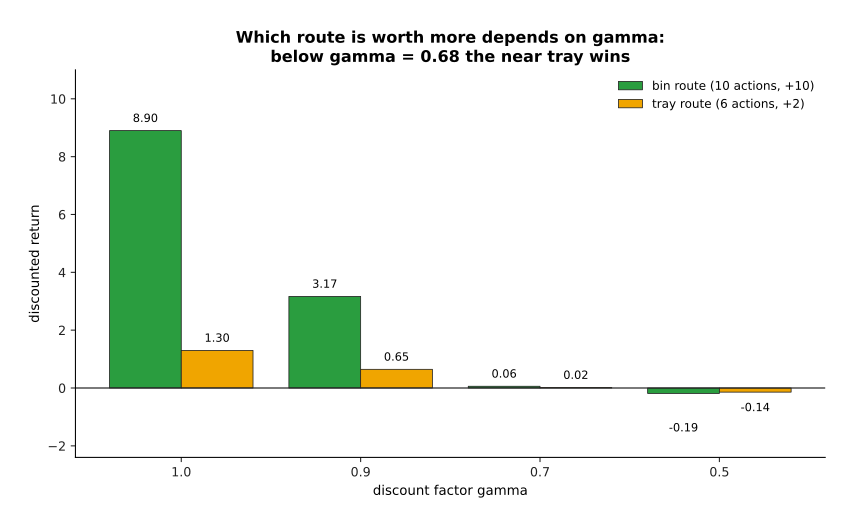
At a gamma of 0.9 the bin route is worth 3.17 and the tray route is worth 0.65. At a gamma of 0.5 the bin route is worth minus 0.19 and the tray route is worth minus 0.14, so the tray has become the better choice. The two routes are worth exactly the same at a gamma of 0.68. Below that value the four extra actions cost more than the extra payment is worth. Choosing gamma is therefore part of saying what you want, rather than a small technical detail. Values from 0.95 to 0.99 are usual, and everything below this point uses 0.95.
2. The policy and the value function#
The words above describe the problem. The two words in this section describe what a reinforcement learner actually builds and keeps.
The first is the policy. A policy chooses the action. It takes a state and gives back a chance for each of the available actions. On a real robot the policy is a neural network whose input is the camera picture and the joint angles, and whose output is the next movement. In this small world the policy is a table with 50 rows and seven columns. The picture below shows three rows of that table, drawn as bar charts, before and after training.
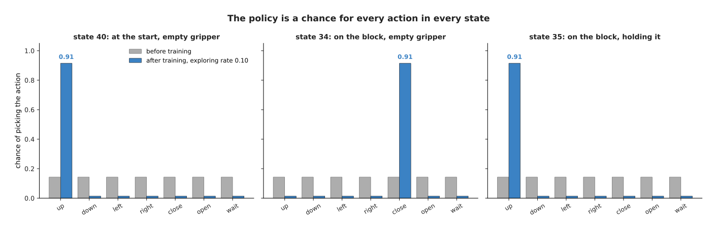
Before training every action has the same chance, which is one in seven, or about 0.14. After training one action in each of those states holds a chance of 0.91, and the remaining 0.09 is shared between the other six so that the learner keeps trying them occasionally.
The second word is the value function. A value function takes a state and gives back one number. That number is the discounted return the learner expects to collect from that state onwards, if it keeps following its current policy. A value is a prediction rather than a payment. A reward says what just happened, and a value says what the future is worth from here. The picture below writes the exact value into every square.
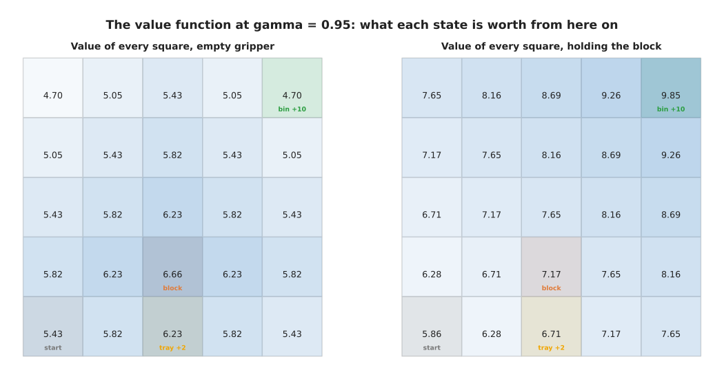
The start square is worth 5.43. The block's square is worth 6.66 with an empty gripper. The bin's square is worth 9.85 once the block is held, because opening the gripper there collects the payment immediately.
The policy and the value function are tied together. Once you know what every state is worth, choosing an action becomes easy, because you take the action that leads to the most valuable state. That is why the arrows in the next picture always point towards larger numbers.
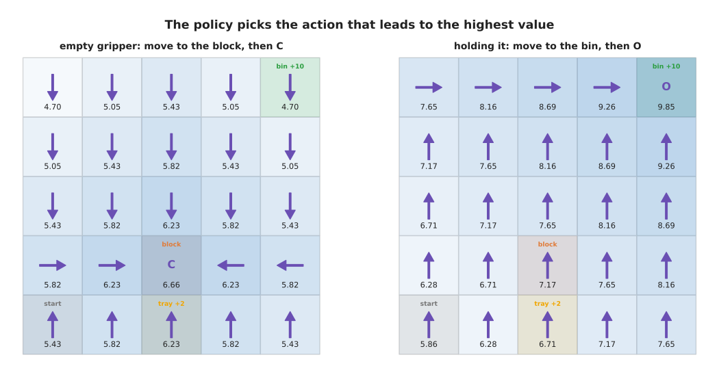
Every arrow leads towards the block while the gripper is empty, and towards the bin while the block is held. The letter C marks the squares where the policy closes the gripper, and the letter O marks the squares where it opens it.
The difference between the two is worth stating plainly. The policy answers the question "what do I do now", and the policy is the part that runs on the robot. The value function answers the question "how well will this go from here", and it exists in order to make the policy better. It can do that because the gap between what it predicted and what really happened is the signal that training uses. Some methods learn both of them, some learn only a policy, and some learn only a value function and then read the policy off it. Section 3 does the last of those three.
Because a value is a prediction, you can check it. You run the policy from a state, add up the discounted rewards it really collects, and compare that total with the prediction. The picture below does exactly that for all 50 states, early in training and at the end.
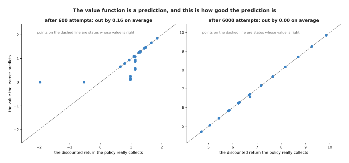
After 600 attempts the prediction is wrong by 0.16 on average over the 50 states. After 6,000 attempts it is wrong by 0.003, which the picture rounds to 0.00, so every point lies on the line.
3. Learning the whole thing from nothing#
Sections 1 and 2 said what gets learned. This section shows it being learned, starting from a table of zeros and using nothing except the rewards that come back.
The method is called Q-learning. It keeps one number for every pair of a state and an action. That number means the value of taking that action in that state and then behaving well for the rest of the attempt. There are 50 states and seven actions, so there are 350 numbers, and all of them start at zero. After every action the learner changes one of those numbers. It moves the number for the action it just took a little way towards the reward it just received, plus the value of the best action in the state it has just arrived in. That one rule is the whole method.
The picture below follows a single one of those 350 numbers. It is the number for state 35, which is the block's square with the block held, and the action "up".
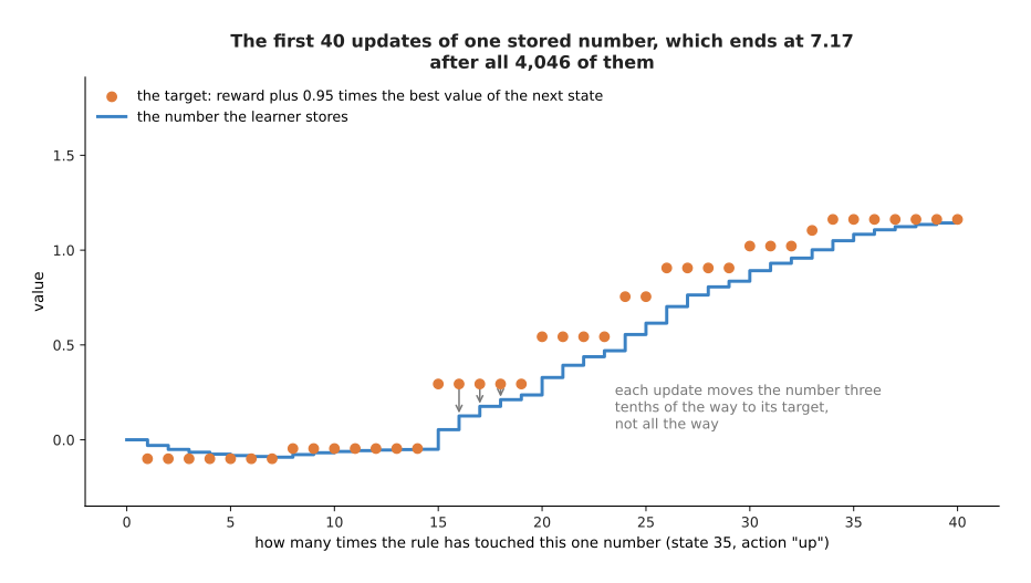
The first time the rule touched that number, the number held 0.000, it aimed at minus 0.100, and it became minus 0.030. The number moves only three tenths of the way towards its target each time. That fraction is the learning rate, and it is the same idea as the step size in gradient descent. It is why the climb is gradual even once the target is correct. The rule touches this one number 4,046 times during the run, and the number ends at 7.17, which is the exact answer.
Running that rule for 6,000 attempts is enough to learn the job. The picture below shows the reward collected in each attempt over the whole run.
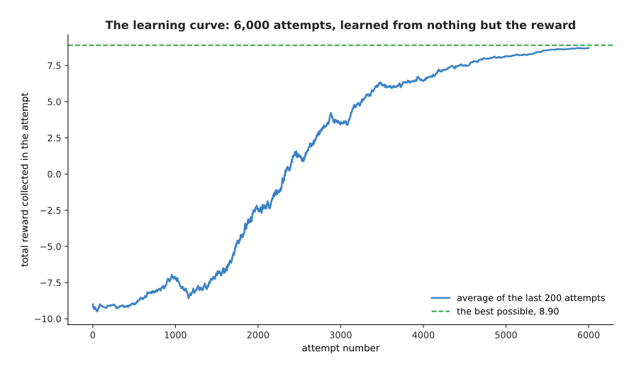
The average reward rises from minus 9.09 over the first hundred attempts to 8.78 over the last hundred. The same run is drawn again below, measured by how often the block really reached the bin rather than by the reward.
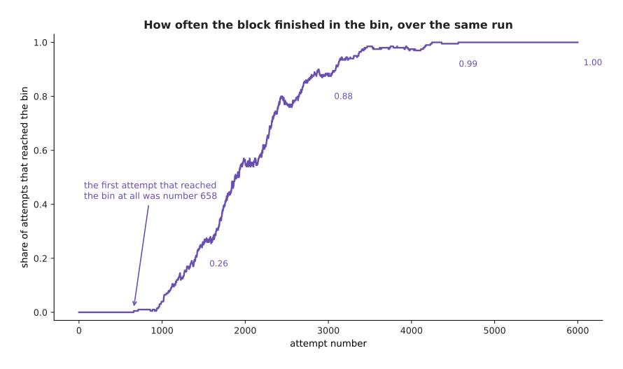
That curve has the shape that nearly every reinforcement learning run has. Nothing happens for a long time, and in this run the first attempt that reached the bin was attempt number 658. Then the curve climbs quickly, because each success tells the learner that a whole chain of earlier states was worth more than it thought. After that the curve flattens, because there is nothing left to improve.
The policy at the start and the policy at the end are easy to compare, because both of them fit on the grid. The picture below draws the chosen action in every square, before training and after it.
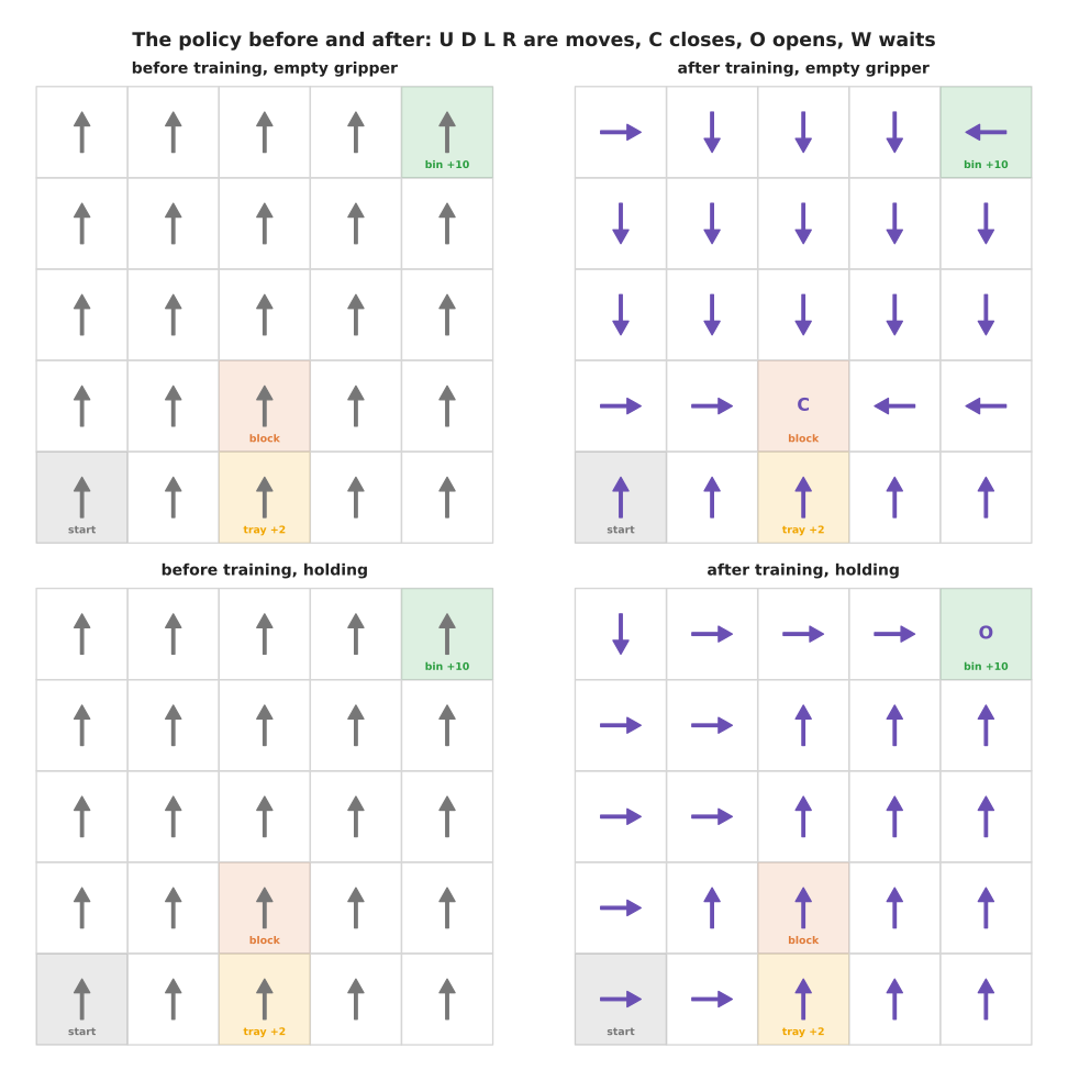
Before training every one of the 350 numbers is zero. All seven actions therefore look equally good, and the learner takes whichever action comes first in the list, which is "up". That is why the untrained grid is covered in identical arrows.
The learned values change in the same way. The picture below shows the learned value of every square with an empty gripper, at three points during the run.
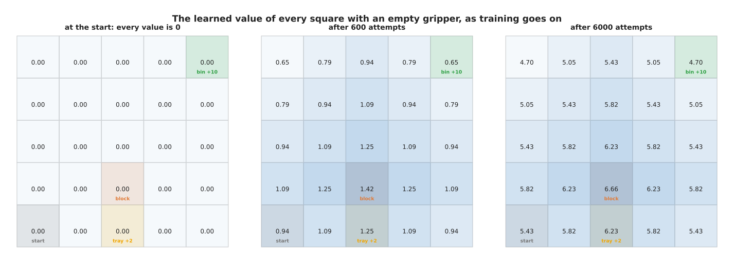
The start square goes from 0 to 0.94 after 600 attempts, and then to 5.43, which is the exact answer.
What happens underneath is that the value travels backwards from the bin. The bin's own square learns its value first. Then the square beside it learns from that one, and so on, until the start square knows what it is worth. The picture below shows that happening in the attempts just after the first success, by grouping the squares according to how far they are from the bin.
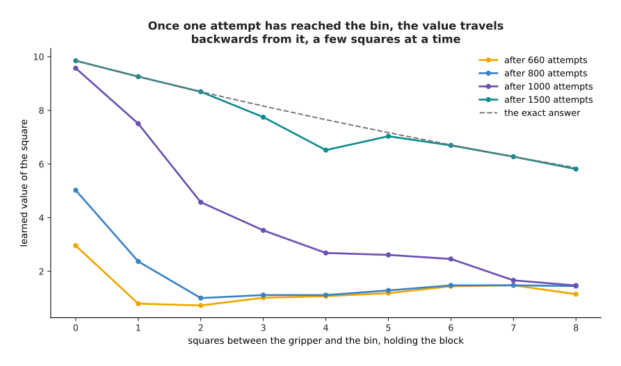
After 660 attempts only the bin's own square has learned anything from that first success, and it holds 2.95. After 800 attempts the bin square holds 5.02 and the squares one step away hold 2.37, so the knowledge has moved one square backwards. After 1,000 attempts it has reached four squares back. After 1,500 attempts the whole line sits on the exact answer. The flat level of about 1.4 at the right of the two earliest lines is not noise. It is what the learner had already worked out about the tray, which it had been reaching for hundreds of attempts.
One state is worth looking at on its own, because it shows that the learner has really learned rather than been lucky. The picture below gives the learned value of all seven actions in state 35, which is the block's square with the block held.
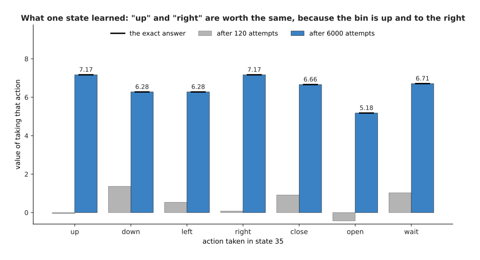
The learner values "up" and "right" at 7.17, "wait" at 6.71 and "open" at 5.18, and every one of those is exactly right. "Up" and "right" are worth the same, which is correct, because the bin is three squares up and two squares to the right, so either move makes the same amount of progress. Opening the gripper is worth the least, which is also correct, because the block would land on an ordinary square and would have to be picked up again. Nobody told the learner either of those two things.
4. Exploring against taking the best answer you know#
Section 3 used one setting without discussing it. That setting decides whether the whole method works at all.
A learner that always takes the action it currently believes is best never finds out about anything better. A learner that always acts at random finds out about everything, and collects almost no reward while doing so. Choosing between those two behaviours is the trade-off between exploring, which means taking an action in order to find out what it does, and exploiting, which means taking the action you already believe is best. The usual way to settle the trade-off is to take a random action with some small chance, and the currently best action the rest of the time.
The picture below compares two sets of runs. In the first set the learner never explores. In the second set it explores on 70 attempts out of every 100.
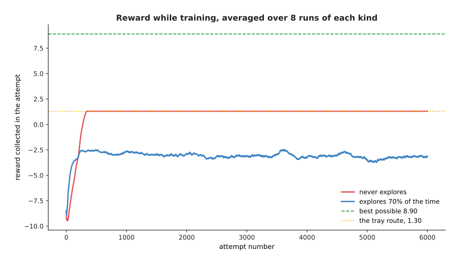
The learner that never explores reaches the value of the tray route within about 300 attempts and then stops improving. The exploring learner stays near minus 3 for the whole run, because 70 out of every 100 of its actions are random and random actions are expensive. That line does not say how good its policy is. It says how much reward was collected while the policy was being found, and those are two different measurements. The next picture puts both of them side by side.
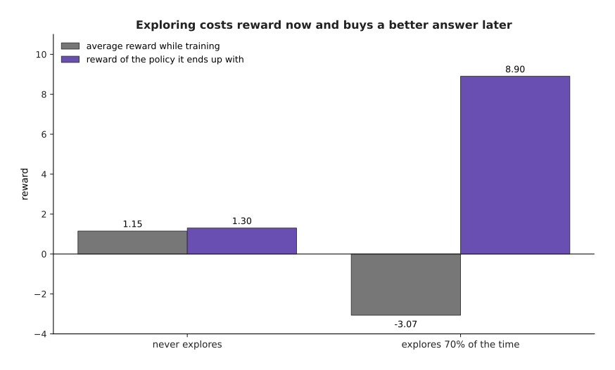
The learner that never explores collects 1.15 on average while training, against minus 3.07 for the exploring learner, so it wins on that measurement. Its finished policy collects 1.30, against 8.90 for the exploring learner, so it loses heavily on the measurement that matters at the end. The exploring learner finishes nearly seven times better.
The reason is visible in the routes the two finished policies take.
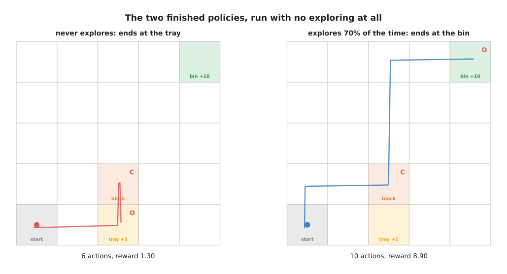
The learner that never explores chooses the tray and never finds the bin, and the bin pays five times as much. The failure here is not bad learning, because its policy is the best possible route to the tray. The failure is that it never saw the bin, so the bin was never part of the problem it was solving. This is the most common way that a reinforcement learning run fails.
Finding the bin at all is the whole difficulty. The picture below counts how many of eight runs of each kind finished with a policy that goes to the bin.
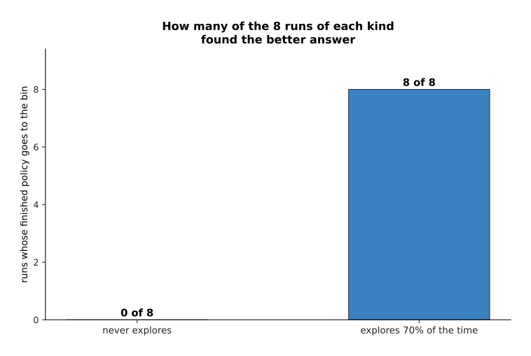
None of the eight runs that never explore ever reached the bin, and all eight of the exploring runs did. When they first reached it varied a great deal, as the next picture shows.
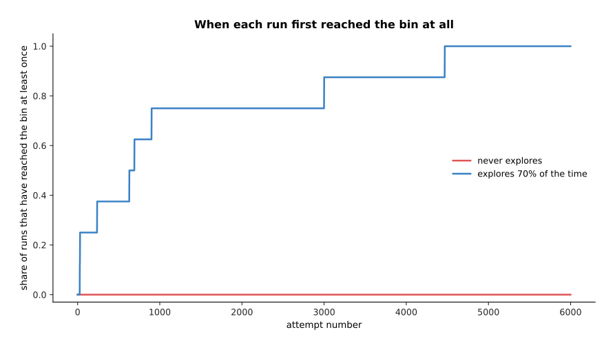
The exploring runs found the bin for the first time somewhere between attempt 26 and attempt 4,468. The runs that never explore never found it at all, so their line stays at zero.
How much exploring to do is not a choice between two options. It is a number between 0 and 1, and the picture below tries seven values of it.
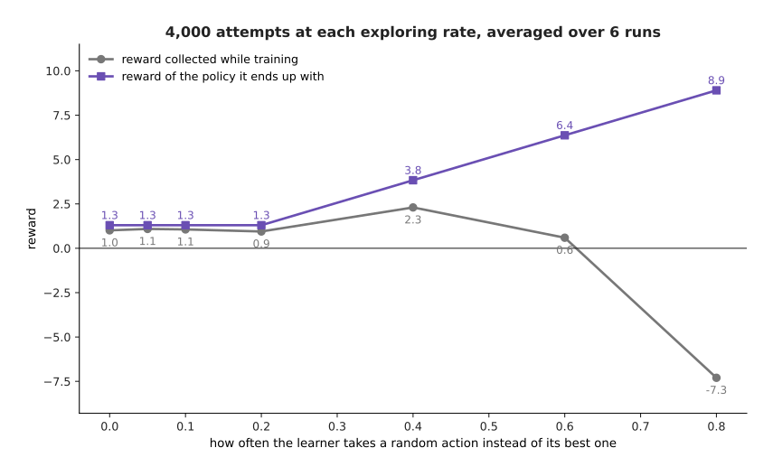
Raising the exploring rate from 0.00 to 0.80 lifts the finished policy from 1.30 to 8.90, and drops the reward collected while training from 1.01 to minus 7.30. The grey line does not fall steadily. A little exploring costs almost nothing here, and at a rate of 0.40 it even collects more than no exploring at all, because it finds the bin. Only a lot of exploring is expensive.
In this world more exploring is always better for the finished policy, because random wandering sooner or later arrives at the bin. That is not true in general. In a world with a thousand states, random wandering finds nothing useful, and the answer is then to explore in a cleverer way or to start from demonstrations given by a person. What is true in general is the shape of the grey line, because exploring is paid for out of the reward collected while training. On a real arm that payment means broken parts and operator time.
5. Whose attempts you learn from, and how big a step to take#
Section 4 was about which attempts get made. This section is about two further questions. The first is whether a learner may use attempts that some other policy made. The second is how far a learner may change itself after reading those attempts.
A method is off-policy when it can learn from attempts made by any policy at all. That includes older versions of itself, and a person driving the arm by hand. Q-learning is off-policy, because its rule asks what the best action in the next state is worth, rather than what the policy that collected the attempt actually did. Any attempt can therefore be stored and used again later. The picture below shows that happening. The table starts empty, and the only input is 1,500 attempts made earlier by a policy that acted completely at random.
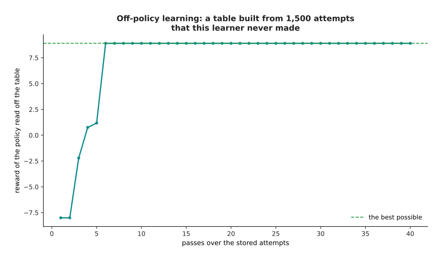
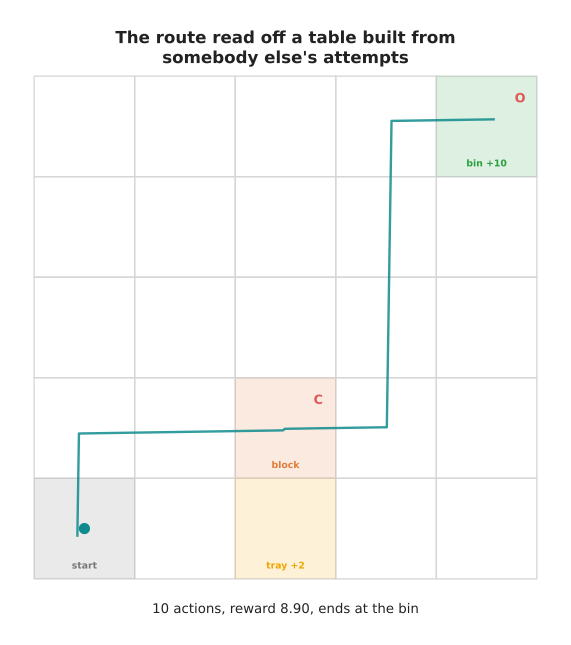
Only two of those 1,500 random attempts ever reached the bin. After one pass over the stored attempts the table gives a policy worth minus 8.00. After five passes it is worth 1.18, which is about the value of the tray. After six passes it reaches 8.90, which is the best possible, and further passes change nothing. The route it finds is as short as the one section 3 learned by trying, although it turns upward one column later.
A method is on-policy when it can only learn from attempts made by the policy it is currently improving. Policy-gradient methods are on-policy. A policy-gradient method changes the policy's numbers directly, in order to make good actions more likely. The size of the change it asks for depends on how likely the policy was to take that action at the time the attempt was made. Once the policy has moved, the stored attempts describe a policy that no longer exists, so they are no longer usable. Handing a policy-gradient method the same stored attempts shows the difference plainly.
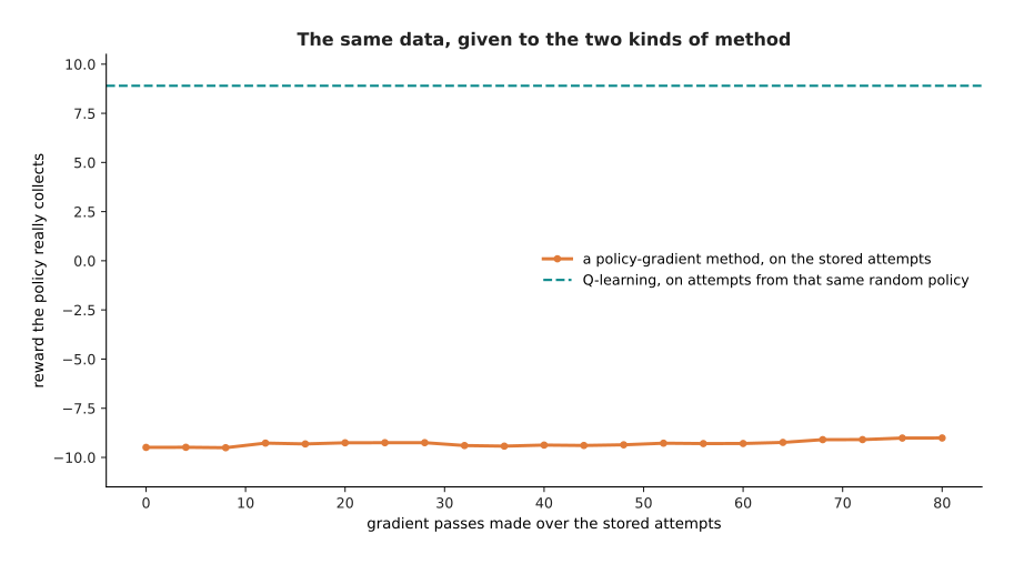
Given 1,500 attempts from the same random policy, the policy-gradient method moves the policy from minus 9.49 to minus 9.01 over 80 passes. Q-learning reached 8.90 on that very same data.
Why would anybody use an on-policy method at all? The answer is that it works directly on the policy, so it can handle actions that are real numbers rather than a short list of choices. An arm needs exactly that, because a joint command is a real number. The price is that every improvement needs fresh attempts, and fresh attempts are the expensive part.
Proximal policy optimisation, usually shortened to PPO, is built to reduce that price. It is the most widely used policy-gradient method. It works in two parts. The first part is to collect a batch of attempts and then improve the policy on that batch several times over, rather than once. The picture below shows what that buys.
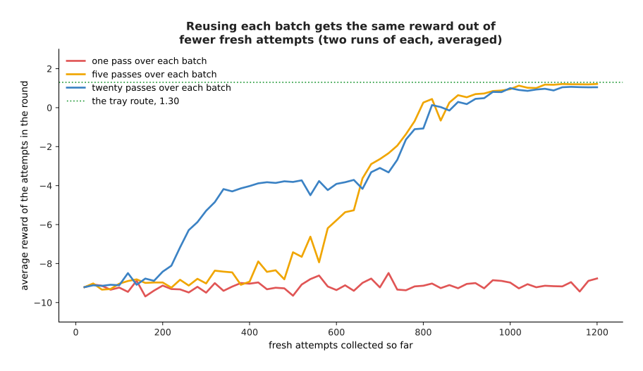
One pass over each batch collects minus 9.11 after 1,200 fresh attempts, which means it has learned nothing at all in that time. Five passes over each batch begin to improve after about 600 attempts. Twenty passes begin to improve after about 200 attempts and arrive at the same place sooner. That is the whole point, because fresh attempts are what a real arm charges you for.
The second part of PPO is a limit, and the limit is needed because of the first part. Improving the policy repeatedly on one batch pushes the policy further and further from the policy that collected it, and the batch then describes something that no longer exists. So PPO refuses to let any action's chance move more than a fixed fraction away from what it was when the batch was collected. It does that by paying the update nothing for a change beyond that band.
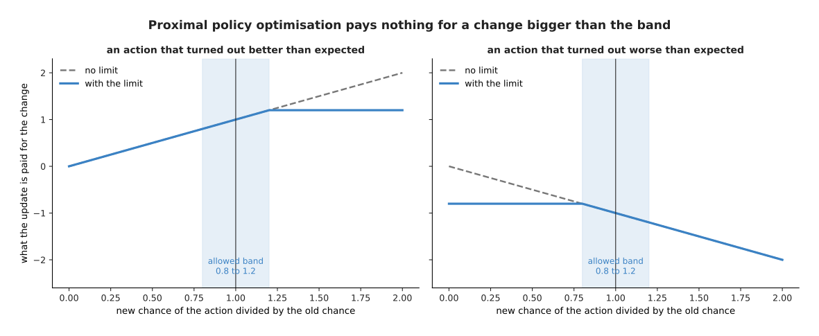
The two panels are the same payment rule, drawn once for an action that turned out better than expected and once for an action that turned out worse. Raising a good action's chance beyond 1.2 times its old value earns nothing extra, so the update stops pushing in that direction.
Take the limit away and the result is a collapse rather than a slow decline. One large step can push an action's chance all the way to certainty, and a policy that only ever takes one action collects no information about any other action.
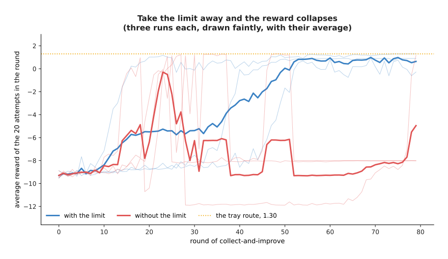
With the limit in place the reward over the last ten rounds averages 0.73, and the best it reaches on the way is 1.05. Without the limit the best it reaches is 1.20 and the reward over the last ten rounds is minus 7.58. Both learners here choose the near tray rather than the bin, for the reason section 4 gave, so the comparison to make is between the two lines rather than against 8.90.
The cause of the collapse is visible in how far the policy moves in one round.
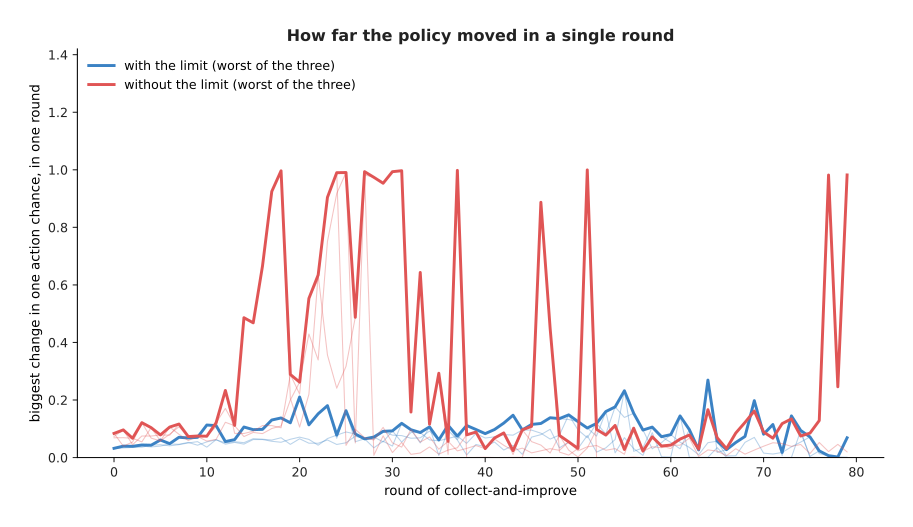
With the limit, no action's chance moves by more than 0.27 in a round. Without it, one chance moves by the full 1.00, which means it goes from impossible to certain in a single round.
6. Why this happens in a simulator, and what the crossing costs#
Every number so far came from a world that costs nothing to run. This section is about what happens when the world is a real arm standing on a bench.
The worked example used 6,000 attempts and 239,361 separate actions, in a world with only 50 states. A real pick-and-place task has a state made of a camera picture and a dozen joint angles, so it needs far more attempts rather than fewer. The picture below shows how many actions each attempt used.
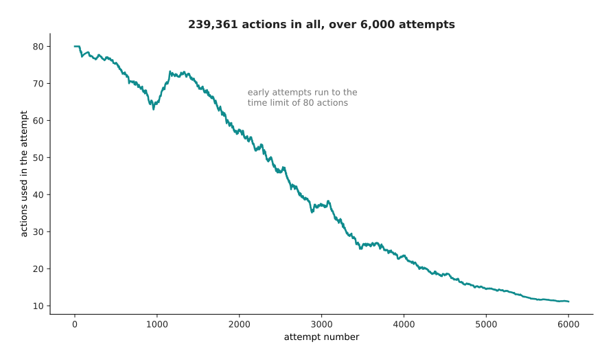
Early attempts use the full limit of 80 actions, because the learner has no idea what to do and the attempt never ends on its own. Later attempts use about ten actions, because the learner goes straight to the bin.
Now take those 239,361 actions as they stand, and allow three seconds for a real arm to carry out one action and be reset when it drops something. The picture below compares the two places the same learning could be done.
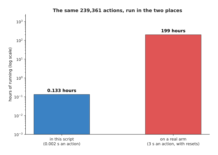
The same 239,361 actions take about eight minutes inside this script and 199 hours on a real arm, which is 8.3 days of continuous running.
That is why reinforcement learning for arms almost always happens in a simulator. A simulator is a program that pretends to be the robot and the table. It can run many copies of the world at once, and it can run each of them faster than real time. Moving the finished policy onto the real arm afterwards is called sim-to-real transfer, where "sim" is short for simulator. The trouble is that the simulator is never exactly right. The friction is wrong, the object is heavier than the model says, and the bench has a fixture bolted to it that nobody put in the simulator. That difference, together with the drop in performance it causes, is called the reality gap.
The picture below shows one policy in both places. The fixture is one square of the table that the simulator did not know about.
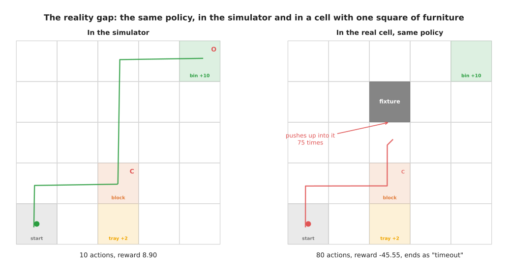
In the simulator the policy reaches the bin in ten actions and collects 8.90. In the cell, the same policy pushes up into the fixture 75 times in one attempt, uses all 80 actions, and collects minus 45.55. That failure has the shape that real failures have. The policy is not confused. It carries out a plan that was correct in the simulator and is impossible in the cell, and because its state never changes it repeats the same action for ever.
Six policies were trained in the perfect simulator, and all six learned the same route. The next picture measures all six in both places.
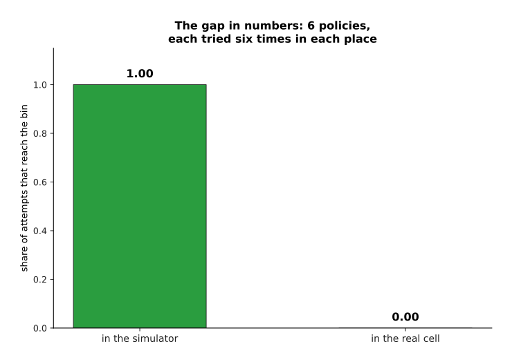
All six reach the bin on every attempt in the simulator, and none of them reaches it even once in the cell.
The usual answer is domain randomisation. It means changing the simulator's settings at random for every attempt, so that the policy has to work across a whole range of worlds rather than one. If the friction, the lighting, the object's weight and the fixture's position are all drawn fresh for each attempt, the policy cannot rely on any of them. The real cell then has a good chance of being one more member of that range. The picture below tries both kinds of policy against each of the eight squares the fixture could stand on.
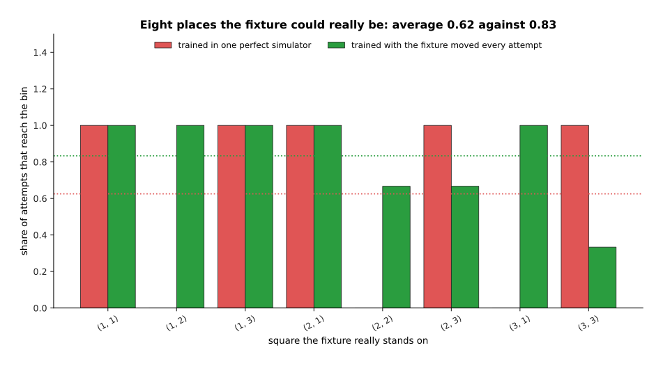
Averaged over those eight squares, the policies from the perfect simulator reach the bin on 0.62 of attempts, and the randomised ones reach it on 0.83. The randomised policies are not better on every square. On two of the eight squares they are worse, and on one of those two they reach the bin on only 0.33 of attempts. What randomisation buys is a better average over the whole range, not a guarantee. The randomised policies also choose a different route.
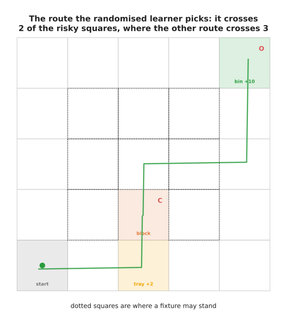
The dotted squares are the ones where a fixture may stand. This route crosses two of them, where the route learned in the perfect simulator crosses three, and one of those three is the square the fixture really stood on in the picture above. The randomised learner did not avoid risk perfectly, because a shorter route is still worth something. It avoided enough of it to survive.
What domain randomisation costs is worth saying plainly, because it is often described as free and it is not. The randomised learner is solving a harder problem, so it needs more attempts to learn.
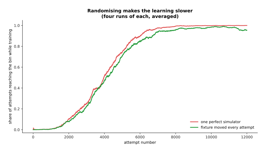
Over the whole run the randomised learner reaches the bin on 0.649 of its training attempts, against 0.679 for the learner in the perfect simulator. There is also a second cost to look for, which is whether the randomised policy is worse back in the easy world.
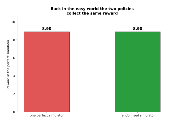
In this small world the randomised policy loses nothing when there is no fixture, because several routes have the same length and it simply picks a safer one. In a harder world there is usually a real price, and the policy that handles every friction setting is a little worse at the one setting the bench turns out to have. How wide to draw the range is a judgement, and it can be settled honestly only by measuring on the real arm.
7. Where to read next#
- Rewards, preferences and verifiers is the next page, and it answers the question this page left open, which is where the reward number comes from when nobody can write one.
- Behaviour cloning and action chunks shows the other way to get a policy for an arm, which is to copy demonstrations rather than to try things.
- World models explains how a learned model of what happens next can take the place of the simulator this page used.
- Post-training a language model shows the same machinery used on text, where one episode is one answer.
- Reinforcement learning policies is the catalogue page for arms, and it says which jobs are really done this way.
- Learned dynamics models lists the real models that predict what the world does next.
8. Using it in Python#
Sections 1 to 3 built a state, an action, a reward and a value table by hand. This section shows the same loop written in NumPy, on the same small world the pictures use. Nobody writes this rule themselves for a real robot, but a table this small makes the rule visible.
import numpy as np

BLOCK, TRAY, BIN = (3, 2), (4, 2), (0, 4)              # section 1's little world
MOVE = [(-1, 0), (1, 0), (0, -1), (0, 1)]              # up, down, left, right

def step(state, action):
    """The world answers: the next state, the reward, and whether it has ended."""
    r, c, h = state // 10, (state // 2) % 5, state % 2  # row, column, holding
    nr, nc, nh, reward, done = r, c, h, -0.1, False     # every action costs 0.1
    if action < 4:
        dr, dc = MOVE[action]
        if 0 <= r + dr < 5 and 0 <= c + dc < 5:         # a wall leaves it where it was
            nr, nc = r + dr, c + dc
    elif action == 4:                                   # close the gripper
        reward -= 0.05
        if not h and (r, c) == BLOCK:
            nh = 1
    elif action == 5:                                   # open it
        reward -= 0.05
        if h:
            if (r, c) == BIN:
                reward, done = reward + 10.0, True
            elif (r, c) == TRAY:
                reward, done = reward + 2.0, True
            else:
                reward, nh = reward - 1.0, 0            # the block is dropped
    return (nr * 5 + nc) * 2 + nh, reward, done

n_states, n_actions, gamma, alpha = 50, 7, 0.95, 0.3
Q = np.zeros((n_states, n_actions))                    # section 2's value table
rng = np.random.default_rng(7)

for attempt in range(6000):
    eps = 1.0 - 0.95 * attempt / 5999     # section 4: explore a lot, then less
    state, seen = 40, []                  # state 40 is the start square
    for _ in range(80):                   # give up after 80 moves
        if rng.random() < eps:
            action = int(rng.integers(n_actions))      # explore
        else:
            action = int(np.argmax(Q[state]))          # exploit
        nxt, reward, done = step(state, action)        # the world answers
        seen.append((state, action, nxt, reward, done))
        state = nxt
        if done:
            break
    for st, ac, nxt, reward, done in reversed(seen):   # section 3's rule, last move first
        target = reward if done else reward + gamma * Q[nxt].max()
        Q[st, ac] += alpha * (target - Q[st, ac])

print(Q[40].max())        # 5.43, the value of the start square
print(np.argmax(Q[40]))   # 0, which is "up"
Both printed numbers appeared in sections 2 and 3. The first one can also be checked by hand, because the best attempt pays 9.85 ten steps away and costs about 0.1 a step before that.
One part of the loop is worth a second look. The whole attempt is remembered in the
list called seen, and the rule is then applied to its moves in reverse order, with
the last move first. Applying the rule as you go also works, but it learns far more
slowly, because the reward at the bin then travels back by one square per attempt
instead of travelling the whole way at once.
A library does everything in that program except the update rule itself. For a real
arm the value table becomes a neural network, so Q[state] becomes a forward pass
and the update becomes a loss and a gradient step. Stable-Baselines3 and CleanRL
both ship proximal policy optimisation ready built. The step function above is the
interface that Gymnasium asks a simulator to provide. MuJoCo and Isaac Lab provide
the arm and the table.
What you still decide is everything this page argued about. You choose the discount factor, and section 1 showed that it changes which behaviour counts as best. You choose how much exploring to do, and section 4 showed that it decides whether the good answer is ever found. You choose how far the policy may move in one step. Above all you choose the reward, and the next page is about how often that choice is the thing that goes wrong.