The four pages before this one all assumed that a person can do the task, because a copying policy has nothing to learn from otherwise. So this page answers one question: how can a robot arm learn a movement that nobody can show it, by trying again and again and being told how well each try went? That way of learning is called reinforcement learning, and the model it produces is a reinforcement learning policy.
The page is for a reader who has read how a model learns and, ideally, behaviour cloning. Behaviour cloning copies a person, whereas reinforcement learning does not need a person to do the task at all, because it needs a way to score each attempt instead. Every new word is explained where it first appears.
Contents#
- What it is
- What goes in and what comes out
- How it works inside
- How it is trained
- Well-known models and methods
- Where this is going
- Where to read next
1. What it is#
The introduction said that the arm learns by trying, so here is that idea in one sentence. The arm tries a movement, a program gives the attempt a score, and the model is changed a little, so that high-scoring movements become more likely next time.
The score is called the reward, and it is a number that a person writes a rule for, such as "1 if the peg is in the hole, 0 if it is not". The model that picks the movements is called the policy, as it is on every page in this chapter. The process of trying, scoring and adjusting, over and over, is called reinforcement learning, which is often shortened to RL. The word "reinforcement" means that actions which led to a good score are made stronger.
For example, think of a child learning to throw a ball into a bin, where nobody explains the angle of the arm or the force of the throw. The child throws, sees whether the ball went in, and throws again a little differently. So after many throws the child is good at it, and the child needed only one piece of information each time, which was in or out.
Reinforcement learning works the same way, but with two differences. It needs far more tries than a child does, often millions of them. And the rule for the score has to be written down exactly, because the computer follows it exactly.
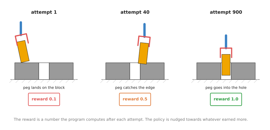
So the picture shows three attempts from early, middle and late in training. The first attempt misses and scores low, while the last one puts the peg in the hole and scores 1.0. Those numbers are an example of a reward rule, and not a measurement.
2. What goes in and what comes out#
Section 1 introduced the reward, so this section shows where it sits among the other numbers. A reinforcement learning policy for an arm takes in a description of the current moment, which is called the observation, and for an arm it can include:
- the joint angles and how fast each joint is turning
- the position of the gripper
- readings from a force sensor at the wrist, which measure how hard the arm is pushing on something
- sometimes camera pictures, although many policies use simple numbers instead, because pictures make learning much slower
Then it gives back one action, which is a small movement command for the next moment, such as "move the gripper 2 mm down and 1 mm left". The policy is asked again many times a second, so the arm moves in many small steps.
The table below shows one concrete example of all of these. Read each row as one input or output of the policy.
| What it is | An example for pushing a peg into a hole | |
|---|---|---|
| In | joint angles and speeds | six angles and six speeds |
| In | gripper position | where the peg tip is, in millimetres |
| In | force at the wrist | how hard the peg presses on the block, and in which direction |
| Out | an action | a small push: 2 mm down and 1 mm left, repeated many times a second |
| Used only in training | the reward | 1.0 when the peg is fully in, less when it is close |
Notice that the reward is not an input to the finished policy. It is only used while training, to decide how to change the policy.
3. How it works inside#
Section 2 said what goes in and out, and this section says what sits between them. Inside, the policy is usually a small neural network. A neural network is a calculation with many adjustable numbers, and Chapter 1 explains it in inside a neural network. For a task that uses simple numbers as input, the network can be small, with only a few layers.
So what makes reinforcement learning different is not the network. It is the loop around the network during training, and here is that loop.
- The arm, which is usually a simulated one, starts in some position.
- The policy looks at the observation and picks an action. While learning, it adds a little randomness, so that it sometimes tries something new, and this is called exploration.
- The arm makes that movement, and the simulation works out what happened.
- The program computes the reward for what happened.
- This repeats until the attempt ends, either because the peg goes in or because time runs out, and one whole attempt is called an episode.
- After many episodes, a learning method looks at which actions came before high rewards and which came before low ones. Then it changes the network's numbers, so that the good actions become more likely.
- Back to step 1, with the slightly better policy.
Step 6 leaves one thing open, and that one thing is what separates the two algorithms section 5 recommends most. Some methods learn from a batch of attempts once and then throw the batch away, which is what PPO in sub-section 5.1 does. Others keep every attempt and train on it again and again, which is what SAC in sub-section 5.2 does. The rest of the loop is the same either way.
Many methods also train a second network, called a critic or a value function, which learns to guess how much reward is still to come from the current moment. This helps, because the real reward often arrives only at the very end, so the critic lets the learner tell early on whether things are going well. All three of the methods recommended in sub-sections 5.1 to 5.3 train one.
One difficulty in that loop is important enough to need a name. When the reward only arrives at the end, the learner has to work out which of hundreds of small actions deserved the credit. This is called the credit assignment problem, and it is one reason reinforcement learning needs so many tries. Sub-section 5.4 describes a method that attacks it directly, by reading the change in the critic's score from one moment to the next as the measure of whether the action in between helped.
4. How it is trained#
Section 3 described a loop that runs many times, and this section says where those runs happen. Reinforcement learning makes its own data by trying things, so it does not need recorded demonstrations. But it needs a very large number of tries, often in the millions. A real arm cannot do millions of tries, because it would take years, and it would wear out or break things. So almost all reinforcement learning for arms happens in a simulator, which is a program that works out how a virtual arm and virtual objects move and bump into each other. A simulator can run thousands of virtual arms at once, much faster than real time, on a graphics card.
But this creates a new problem, because the simulator is never exactly like the real world. Friction, weight, springiness and camera pictures are all a little wrong, so a policy that learned in the simulator can fail on the real arm, and this gap is called the sim-to-real gap.
The most common fix for that gap is called domain randomisation. Instead of building one very accurate simulated world, you train in thousands of slightly different ones. Each one has a different table colour, different lighting, a different friction, a slightly different mug size, or a camera in a slightly different place. The policy has to work in all of them, so the real world is, with luck, just one more variation it has already met.
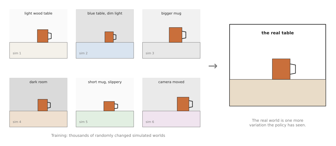
The picture shows six of the randomised training worlds on the left, each with one thing changed, and the real table on the right.
But there are two other ways to get the practice.
- Offline reinforcement learning learns from a fixed pile of recorded attempts, without practising at all.
- Real-world reinforcement learning practises on the real arm, but only for a short time. It usually starts from a policy that already works a little, which is often one trained by copying. A person watches and can take over when the arm goes wrong, and those corrections help the learning.
The second of these is where much of the useful work happens in 2026, and the learned methods document describes the evidence.
5. Well-known models and methods#
The pages before this one each end with a shelf of models you can download. This page cannot, and saying so plainly is the most useful thing in it. Reinforcement learning is the one method in this chapter where you train rather than download, because a finished policy belongs to one reward rule, one simulated world and one robot, so nobody publishes it for you to pick up. The names worth knowing are therefore the learning methods and the libraries that implement them, and the rest of this section helps you choose one of each.
Read the table as a shortlist of choices rather than of products. The left column names the method and says how current it is. The right column holds everything you need in order to compare them: what the thing is, what it is best at, how much practice it needs, the licence of the code you would run, and when to pick it. These are methods, so where a model's size would normally go you get the amount of practice instead, which is the cost that decides most projects. Each licence is the licence of the code you would actually run, read from that project's own licence file, because a method itself has no licence.
| Name | What decides it |
|---|---|
| PPO, most used in 2026 | PPO is an algorithm from 2017, and it is best where a simulator runs many arms at once. It needs millions of steps of practice. The code you would run is Stable-Baselines3, which is MIT. Pick it when you can simulate the task and score it. |
| SAC, most used in 2026 | SAC is an algorithm from 2018, and it learns from as few attempts as possible. It needs far fewer steps than PPO, because it replays a store of past ones. The code you would run is Stable-Baselines3, which is MIT. Pick it when every attempt costs real time. |
| HIL-SERL, most used in 2026 | HIL-SERL is a system you can run, published in 2024, and it improves a half-working policy on the real arm. It needs one to two and a half hours of real practice. Its code is Apache-2.0, and it ships inside LeRobot. Pick it when you have the arm, and a person to watch it. |
| Recap, in π*0.6, worth betting on | Recap is a method from 2025, and it polishes a large pretrained policy. The practice it needs is not stated. No code or weights were released, so you cannot pick it today, but it is worth following. |
| Offline: IQL and CQL, historical | IQL and CQL are algorithms that learn from recordings without practising, so they need no practice at all. Their licence was not checked. Pick them almost never now, and sub-section 5.5 says why. |
| The landmark systems, historical | These are published results from 2018 to 2023, and they show what the method has achieved. They took weeks of real collection, or none at all, and their licences are various. Pick them when you are reading rather than building. |
5.1 PPO, for practising in a simulator#
Most used in 2026 when the practice happens in a simulator, because it stays stable while thousands of simulated arms practise at once.
Millions of steps of practice, an NVIDIA card to run a simulator fast enough to produce them, and MIT for the Stable-Baselines3 code you would run.
PPO stands for Proximal Policy Optimization, and OpenAI published it in July 2017 in Proximal Policy Optimization Algorithms.
The one idea PPO is built on is that the policy may only be changed a little at a time. The reason is the one section 3 mentioned: the attempts PPO learns from were made by the policy as it stood a moment ago, so the further the policy moves away from that, the less those attempts say about it. PPO's answer is to put a hard limit on how far one update may move the policy. That limit is the "proximal" in its name, and it is why a PPO run of many hours rarely falls apart.
What that changes inside is small but it decides everything else. PPO trains a critic, which is the second network section 3 described, and uses it to work out the advantage of each action, meaning how much better the attempt turned out than the policy expected at that moment. The update then takes the chance that the new policy would choose that action, divides it by the chance that the collecting policy would have chosen it, and multiplies the result by the advantage. The limit is applied to that division: once the ratio leaves a narrow band around one, the update stops rewarding any further movement in that direction. So the batch is worth a few passes of learning, and then the policy has moved as far as it is allowed and the batch is thrown away.
What that buys is stability and scale. The limit does not care how many arms filled the batch, so a thousand simulated arms can all pour into one update and the run behaves the same, which is why most large-scale simulation results in this field are PPO results. What it costs is everything the throwing away costs. Each step of practice teaches the policy once, inside those few passes, and is then gone, so the only way to learn a hard task is to produce an enormous number of steps.
On a robot arm that cost is the whole decision. In a simulator running a thousand arms on a graphics card, a discarded step costs almost nothing, so the stability is free. On a real arm, a step is a second of real movement with somebody standing by to put the block back, so discarding it is the most wasteful thing you could do with it. That is why nobody runs plain PPO on real hardware, and why the two sub-sections after this one both keep their attempts instead.
So pick PPO rather than SAC in the next sub-section when attempts are cheap, because what you want in a simulator is a run that does not collapse overnight.
The simulator, not the algorithm, is what you have to choose carefully. Isaac Lab (BSD-3) and MuJoCo Playground (Apache-2.0) are where large-scale practice happens, and both want an NVIDIA card, so on an Apple Silicon Mac you are limited to plain MuJoCo on the processor and to small tasks. Note also that Isaac Gym, the simulator behind a great many older papers, is officially no longer supported, and Isaac Lab replaced it, so a tutorial built on Isaac Gym is out of date. What most often goes wrong is not the algorithm but the reward.
The library for the algorithm itself is
Stable-Baselines3, which is MIT and
installs with pip install "stable-baselines3[extra]". The code below trains on
sixteen copies of a simulated pushing task from
panda-gym (MIT,
pip install panda-gym).
import panda_gym                       # registers the Panda tasks with gymnasium
from stable_baselines3 import PPO
from stable_baselines3.common.env_util import make_vec_env

# Sixteen copies of the task in one process. PPO learns from all of them together,
# which is the whole reason it suits a simulator.
env = make_vec_env("PandaPush-v3", n_envs=16)

# MultiInputPolicy because this task's observation is a dictionary, holding the
# arm's state, the object's position and the goal separately.
model = PPO("MultiInputPolicy", env, n_steps=2048, batch_size=64, verbose=1)
model.learn(total_timesteps=2_000_000)
model.save("ppo_panda_push")
Stable-Baselines3 gives you the algorithm. n_steps=2048 and batch_size=64 are its
own defaults for PPO, and with sixteen copies of the task each update learns from
32,768 steps of experience. What panda-gym gives you is the simulated arm, built on
the PyBullet physics engine, the task and, most importantly, the reward. On your own
task you write that reward yourself. For a wider set of manipulation tasks,
robosuite (MIT) provides them on
MuJoCo instead, and it runs on Apple Silicon because MuJoCo does.
5.2 SAC, for when every attempt is expensive#
Most used in 2026 when attempts are expensive, because it reuses old attempts instead of throwing them away.
Far fewer steps of practice than PPO, a laptop if the observations are plain numbers, and MIT for the Stable-Baselines3 code you would run. The store of past attempts needs memory of its own, and that is the part that grows.
SAC stands for Soft Actor-Critic, and researchers at the University of California, Berkeley published it in January 2018 in Soft Actor-Critic: Off-Policy Maximum Entropy Deep Reinforcement Learning with a Stochastic Actor.
The one idea SAC is built on is that you can learn something that does not belong to the current policy. What SAC's critic learns is the value of a situation together with a movement: if you are here and you do this, how much reward follows. That statement is about the world, not about the policy, so it stays true no matter which policy made the attempt. PPO's limit exists because its update is a statement about the policy that collected the batch. SAC has no such tie, so an attempt made an hour ago by a much worse policy is still perfectly good data.
What that changes inside is that the attempts are kept. Every step the robot takes goes into a store called a replay buffer, and each update draws a random handful out of the store rather than using what just happened. The same movement is therefore learned from many times, in different combinations, which is the saving in attempts the table credits it with. The numbers in Stable-Baselines3 say the difference plainly: SAC's buffer holds 1,000,000 past steps by default and it trains on a batch of 256 of them after every single step the robot takes, where PPO waits for 2,048 fresh steps and then discards them.
Keeping the attempts brings its own problem, and most of SAC's parts exist to handle it. A critic that is asked to score movements nobody has tried lately drifts towards being over-confident about them, and the actor then goes and performs them. So SAC trains two critics and believes the lower of their two scores, which means a score has to be over-confident in both of them before it is acted on. It keeps a slowly updated copy of them, so the target a critic is trained towards does not move as fast as the critic does. And it pays the policy a little for keeping some randomness, with the size of that payment tuned automatically, which stops the policy settling early on the first thing that half worked. Where PPO's correctness came from one limit, SAC's comes from this stack, and each piece of it quietly ruins a run when it is wrong.
On a real arm the difference is exactly the number of attempts you have to pay for. Suppose you can afford two hundred attempts before the hardware or your patience runs out. SAC will have learned from each of those attempts many times over by the end, while PPO will have learned from each of them once and discarded it. That is the whole reason a real arm gets SAC and a simulator gets PPO. The same property has a limit worth knowing: a million camera pictures will not fit in a laptop's memory, which is one reason these policies often take plain numbers as input rather than pictures, as section 2 said.
Pick SAC rather than PPO when you count your attempts, which means on a real arm, or in a simulator too slow to run many copies. What it costs you is the complexity above, and getting a tested implementation is the real value of the library here.
The library is Stable-Baselines3 again, and the simulated arm below is panda-gym.
import gymnasium as gym
import panda_gym
from stable_baselines3 import SAC

env = gym.make("PandaPickAndPlace-v3")
model = SAC("MultiInputPolicy", env, buffer_size=1_000_000, batch_size=256, verbose=1)
model.learn(total_timesteps=500_000)
model.save("sac_panda_pick_and_place")

observation, info = env.reset()
# deterministic=True switches off the exploring randomness, so the trained
# policy does its best instead of trying something new.
action, _ = model.predict(observation, deterministic=True)
observation, reward, terminated, truncated, info = env.step(action)
Look at total_timesteps=500_000 before you believe this is cheap. If the arm
decides twenty times a second, half a million steps is about seven hours of
continuous motion, and on a real arm it is far more, because somebody has to put the
object back after every attempt. What you have to supply for your own robot is a
simulator of that arm, accurate enough to train against, plus the randomisation of
section 4 and usually a short spell of real practice at the end. That last step is
the subject of the next sub-section.
5.3 HIL-SERL, for learning on the real arm#
Most used in 2026 for work on a real arm, and the one entry on this page whose published numbers are strong enough to plan around.
One to two and a half hours of real practice, a real arm with a person sitting beside it, and Apache-2.0 for the code, which ships inside LeRobot.
HIL-SERL stands for Human-in-the-Loop Sample-Efficient Robot Learning, and it came from the University of California, Berkeley in 2024 (project page, repository).
The one idea it is built on is that a person watching a robot is worth more as an interrupter than as a demonstrator. A demonstration shows the policy a situation the person chose. A take-over, where the person grabs the controller the moment the arm is about to fail, shows the policy the one situation it actually gets wrong, together with the way out of it. Those are the most valuable steps in the whole run, and they are the ones no amount of demonstrating in advance will produce, because nobody knows in advance where this policy will go wrong.
That idea only works because of SAC's property from the sub-section above. The take-overs were not produced by the policy, so a method that needed its own attempts could not learn from them at all. HIL-SERL therefore runs SAC underneath, and keeps two stores rather than one: a store of prior data, holding the demonstrations and the person's corrective movements, and a store of what the robot has done by itself. Every update draws half its batch from each, which is a published recipe called RLPD, short for reinforcement learning with prior data. The policy's own movements from either side of a take-over go only into the robot's store, so the person's corrections are never confused with the mistakes that provoked them.
Two more parts make it work on real hardware. The reward is not a rule somebody wrote but a classifier trained on the demonstration images beforehand, which looks at the scene and makes a yes-or-no judgement about success, and that is how a task like "the connector is seated" gets a reward at all. And the system runs as two processes: one drives the arm and takes the person's input, the other does the updates and sends new weights over, so the arm keeps moving while the learning happens instead of pausing for every gradient step. The gripper gets its own separate critic, because open and closed is a choice between two things rather than a number to nudge, and treating it as a number works badly.
Pick it rather than training in simulation with PPO because it removes the simulator, which section 4 named as the hardest part to get right. The published result is the reason to take it seriously. HIL-SERL reached 100 per cent success on every task it was tried on, after between one and two and a half hours of training on the real robot, on tasks including seating memory in a motherboard, inserting an SSD and a USB connector, clipping a cable, fitting a timing belt and assembling IKEA panels, where the strongest copying baseline on the same tasks averaged under 50 per cent. That was peer-reviewed in Science Robotics, which is worth saying in a field where most strong numbers are published by the company that produced them.
What it costs you is several hours of a person's time and a prepared robot. Somebody has to sit with the arm throughout, holding the controller. You also need force and speed limits underneath the policy, a way to put the task back to its starting state between attempts, and a reward classifier you trust, and the learned methods document gives the evidence and the practical requirements. One other thing to know: its predecessor SERL is formally deprecated in favour of it, so ignore any tutorial built on SERL.
The original repository is Apache-2.0, read from its licence file, but the version to use is the one inside LeRobot, documented as its reinforcement learning workflow. It runs as two processes.
# The learner holds the policy and does the SAC updates.
python -m lerobot.rl.learner --config_path train_config_hilserl_so100.json

# The actor, in a second terminal, drives the arm and sends its experience back.
python -m lerobot.rl.actor --config_path train_config_hilserl_so100.json
LeRobot gives you the actor-and-learner split, the SAC implementation underneath it
and the gamepad handling. What you supply is that JSON file and the robot. The file
names your arm, your cameras, the reward classifier and an algorithm block whose
type is sac. Before either command runs you record the demonstrations and train
the classifier, which LeRobot does with its own commands. To walk through the whole
workflow without any hardware, the gym_hil
package gives you a simulated Franka arm with gamepad take-overs, in tasks such as
PandaPickCubeGamepad-v0.
5.4 Practice on top of a pretrained policy#
Worth betting on, because the field has largely stopped training policies from nothing, and this is what it does with reinforcement learning instead.
The practice it needs is not stated, there is no machine to put it on and no licence to read, because nothing was released.
The idea is to train a large policy by copying demonstrations, and then let it practise and be corrected rather than collecting more demonstrations. The clearest published instance is π*0.6 from Physical Intelligence, published on 17 November 2025, and its method is called Recap.
The one idea Recap is built on is that you can keep the simple training of a copying policy and hand it the scoring as one more input. Recap first trains a value function, which is the critic of section 3, to say how close a situation is to success. It then uses that value function to work out, for every action already in its pile of data, whether that action moved the situation forwards or backwards, and it reduces the answer to a single yes-or-no flag. The policy is then trained to copy the data as usual, but with the flag given to it alongside the pictures and the instruction. At run time you set the flag to yes, and you get the version of the behaviour that worked. Its name says so: Recap is short for reinforcement learning with experience and corrections via advantage-conditioned policies, and an advantage here is the same quantity PPO used, meaning how much better an action turned out than expected.
That is a different shape from everything above it. PPO and SAC both push gradients through a critic to change the policy, and the policy has one job, which is to produce the best action it can. Recap's policy has two inputs instead, and the hard reinforcement learning work has moved into the labelling of the data. Because of that, three very different kinds of data can go into one pile: the original demonstrations, a person's take-overs in the style of HIL-SERL, and the robot's own autonomous attempts, good and bad. The flag is what tells the policy which parts of that pile to imitate, so bad attempts are useful rather than harmful, which is not true of plain copying.
The problem that shape solves is the one section 3 named. When a long job fails, the mistake that caused it usually happened much earlier than the failure, and working out which action to blame is the credit assignment problem. The value function is Recap's answer to it, because the change in its score from one moment to the next says whether the action in between helped, whatever happened later. On an arm that is the difference between a job of one movement and a job of twenty. A policy that folds a shirt can fail at the last fold because of the way it picked the shirt up, and neither plain copying nor a single score at the end will ever tell it so.
Bet on this rather than on training from scratch because it fixes the thing that copying cannot fix. Demonstrations show what success looks like and never show how to recover from the particular mistakes that your policy makes. It is also where the field's attention has gone, since training a reinforcement learning policy from scratch is now the exception rather than the rule, and this repository's frontier chapter calls demonstrate-then-polish the most important arrival of the year.
What it costs you today is that you cannot have it, because none of it is released, neither the code nor the weights. The figures that exist come from the company itself, and its per-task numbers appear only as bar charts rather than in the text, so read them as a direction and not as a measurement. Its authors also name the limit themselves, which is that the corrections are only as good as a person's judgement about when to step in, and that works for obvious mistakes and not for subtle ones. So there is no code to show here, and the nearest thing you can actually run is HIL-SERL in 5.3, which is the open version of the human-take-over stage. The frontier chapter on foundation models records what was claimed, with its sources.
5.5 Offline reinforcement learning: IQL and CQL#
Historical, kept because it explains a part of the methods above rather than because you should start a project with it.
No practice at all, because it learns from recordings, a laptop if those recordings are plain numbers, and a licence you have to check yourself, since there is no one implementation to point at.
Offline reinforcement learning learns from a fixed pile of recorded attempts and never practises at all, which section 4 listed as one of the three ways to get the practice. IQL and CQL are the two algorithms people name.
Both are built on one idea, which is the far end of the question this page keeps coming back to. SAC kept its attempts and still made new ones, while an offline method keeps the attempts and makes none. That removes the one thing that was keeping the critic truthful. Section 5.2 said that a critic drifts towards being over-confident about movements nobody has tried lately, and SAC caught that drift because the actor eventually tried the movement and the reward came back low. With no new attempts, nothing ever contradicts the critic, so one invented movement with a high score can ruin the whole policy.
The two algorithms attack that from opposite ends, and the difference is worth knowing because it is the same choice every offline method faces. CQL, short for conservative Q-learning, lets the critic score anything but adds a penalty that pushes down the scores of movements the recordings do not contain, so the critic is deliberately pessimistic about the unknown. IQL, short for implicit Q-learning, never asks the question at all: it fits the value of a situation from the outcomes actually recorded there, leaning towards the better ones, and then trains the policy to copy the recorded actions in proportion to how good they looked. So CQL corrects the critic, and IQL never asks it a question it cannot answer.
The reason it is historical is not that it stopped working. Its benchmark suite, D4RL, was formally deprecated, with Minari as its replacement for datasets, and its algorithms were absorbed into the post-training of copied policies, which is sub-section 5.4. Recap's value function is trained exactly this way, from a fixed pile, which is why this sub-section is here at all. So read this branch to understand how a critic can be trained without new attempts, and take its datasets from Minari rather than from a tutorial built on D4RL. Stable-Baselines3 does not implement either algorithm, which is itself a fair guide to how much demand there is.
5.6 The landmark systems#
Historical, and listed because people cite these as the proof that the method works on real hardware, so it is worth knowing what each one actually showed.
Weeks of real collection or none at all, hardware that almost nobody reading this has, and various licences. None of them ships a policy you can download.
QT-Opt (Google, 2018) learned to grasp objects from a bin using several real robot arms at once, collecting attempts over weeks. It showed that learning on real hardware was possible, and how costly it was. Dactyl (OpenAI, 2018, with a Rubik's Cube follow-up in 2019) learned to turn a block in a robot hand's fingers, trained only in simulation with heavy domain randomisation. IndustReal (NVIDIA, 2023) fitted pegs and gears into holes after training only in simulation, transferring to a real Franka arm with no real practice at all, and reaching between 83 and 99 per cent across 600 trials on parts modelled on a standard assembly test board. Its successor FORGE improved gear meshing to 98 per cent and nut threading to 69 per cent while halving the contact forces.
The three sit at three different points on the one question this page keeps coming back to, which is what you do with an attempt once it is made, and that is the most useful thing about reading them together. QT-Opt is the far end of keeping them. It has no network that outputs a movement at all. It learned only a scoring function, which rates a candidate movement given the camera picture, and it chooses what to do by proposing many random candidate movements, keeping the best-scored of them, proposing more near those, and keeping the best again. Because nothing in that depends on which policy made an attempt, every grasp any robot had ever tried stayed useful, which is the only reason a pile collected over weeks was worth having.
Dactyl is the opposite choice. It is PPO, so it discards each batch, and it could afford to because every one of its attempts was simulated. What it added was memory: its policy carries an internal state from one moment to the next, so it can work out from the first part of an attempt what this particular world's friction and weight feel like and adjust inside the same attempt. Its authors report that a policy without that memory, trained on the same randomised worlds, did markedly worse on the real hand. So where domain randomisation alone asks for one policy that is adequate everywhere, memory asks for a policy that works out where it is.
IndustReal is PPO as well, and it is the most useful one to read if you work with an arm, because its three contributions are all about making a simulated reward tell the truth. Its reward is built from a precomputed field of distances to the part's target pose, so the policy is told how far off it is in position and orientation together, rather than from hand-weighted scores for each. Its curriculum lets the peg start anywhere in the full range from the beginning but raises the minimum starting height as the policy improves, which stopped the policy overfitting to easy, nearly finished insertions. And its policy update checks how far the simulated parts passed through each other and discounts the attempts where they passed through a lot, because a policy will happily learn to push a peg through solid metal if the simulator lets it.
Read IndustReal's caveats rather than its headline, because they say what the method cannot yet do. Its authors deliberately used no force sensor at all, working from vision and joint positions, on the grounds that such sensors are costly, noisy and fragile. The clearances were half a millimetre, which is much looser than a real electrical connector. And none of it is deployed in a factory. None of these four systems ships a policy you can download, which is the point section 5 opened with.
5.7 How to choose#
Before choosing anything here, check that you need this method at all, because most arm tasks do not. If a person can demonstrate the task, the earlier pages in this chapter are far less work for the same result.
When you do need it, the default is not to train from nothing. Train a copying policy first, then improve it on the real arm with HIL-SERL, which is sub-section 5.3. That is the one recipe here with published numbers strong enough to plan around, and it needs no simulator.
Three things change that answer.
If nobody can demonstrate the task at all, you have nothing to improve, so you train in simulation. Use PPO from 5.1 with a simulator that runs many arms at once, and expect the simulator and the reward to take more of your time than the learning does.
If attempts are expensive, because the simulator is slow or the practice is on the real arm, use SAC from 5.2 instead of PPO, because replaying old attempts is the whole point of it.
If you are learning the subject rather than shipping a robot, install Stable-Baselines3 with panda-gym and read the SAC implementation. It is MIT, it runs on an Apple Silicon Mac, and watching a simulated arm fail for an afternoon will teach you more about reward design than reading does.
Leave 5.4, 5.5 and 5.6 out of the decision. One is not released, and the other two are there to be read.
6. Where this is going#
Section 5 described the methods as they stand, and this section is about where they are heading. Four kinds of statement appear below, and they carry different weight. A demonstration is a recording of something working once, under conditions the publisher chose. A product announcement says that something can be downloaded or bought, so you can check it yourself. A research result is a measured number under a stated protocol. A projection is a claim about a date that has not arrived, and it is the weakest. Where a sentence below is my own expectation rather than somebody's claim, it says so. Book 3's what is coming to robot arms uses the same four words across the whole field.
6.1 How it got here#
The method's position has turned over completely. Between 2018 and 2023 reinforcement learning was how a robot was supposed to learn a hard contact task, and the landmark systems in sub-section 5.6 were the evidence for that. Then copying demonstrations turned out to be much less work for anything a person can show, which is most arm tasks. So reinforcement learning stopped being the way a policy is trained and became the stage that comes after one. HIL-SERL in 2024 and Recap in 2025 are both that stage. The algorithms themselves changed very little, and what changed is what they are pointed at.
6.2 Where it is used in industry today#
It is used far less on real arms than the volume of research about it suggests, and that gap is the most useful thing to understand on this page. There is no downloadable reinforcement learning policy for an arm, by construction, as section 5 opened by saying. No vendor has published how many arms at a named customer site are driven by a practised policy, how many hours they ran, or how often a person had to step in. The clearest published success of practice-in-simulation on real hardware is not manipulation at all but legged walking, in a 2019 result in Science Robotics on the ANYmal robot, which trained in simulation and transferred to the machine. The reason that worked is worth taking with you. Walking forwards without falling over is easy to write a score for, and a leg swinging through air is far easier to simulate than a peg entering a hole. Neither condition holds for assembly.
What is checkable and genuinely useful is the open tooling, and all of it is recent. HIL-SERL ships inside LeRobot with a documented workflow under Apache-2.0, and gym_hil lets you rehearse it without hardware. Isaac Lab is where large-scale simulated practice happens. LeRobot's version 0.6.0 of 6 July 2026 added two reward models as downloadable policies, alongside three world models, and a reward model is a separate model that scores whether an attempt is going well. Those are product announcements, and you can test each one by fetching it. None of them is a deployment.
6.3 What is being worked on right now#
The front has moved to practising on top of a policy that already half works, rather than learning from nothing. Sub-section 5.4 described the clearest instance, which is Recap inside π*0.6 from Physical Intelligence. Read that as a research result published by the company that made it, with its per-task figures given as bar charts rather than in the text and no code or weights released, which is about as weak as a research result gets while still being one.
The same shape is now being tried in the open, on top of a model you can download. ForceRFT, submitted in September 2026, freezes a SmolVLA policy trained on demonstrations and learns a small correction on top of it from the force readings at the wrist. The corrections come from two sources, which are a person's take-overs and the robot's own attempts that the system could verify, and the authors are careful to keep the credit from crossing between the two. They report higher autonomous success than both a demonstration-trained policy and a correction learned by copying, on plug insertion, ring-on-peg assembly and whiteboard wiping. That is a research result on real hardware. It matters here because it is the Recap idea built on an Apache-2.0 model that anybody can fetch, so it is the first version of this a reader of this page could reproduce.
The reward is turning into a model rather than a rule somebody writes. HIL-SERL already does this, because its reward is a classifier trained on the demonstration images, and LeRobot has now made reward models a downloadable category of their own. The reward and progress models page covers them. This is the part of the method where the real work is, because section 4 showed that producing the practice is mostly a matter of buying graphics cards, while deciding whether an attempt succeeded is not.
Practice is also being moved off the real arm and out of the hand-built simulator, into a model that learned the physics from recordings. LeRobot shipped three such world models with pretrained checkpoints in the same release, and Book 3's frontier chapter measures the share of robotics abstracts mentioning a world model rising from 2.39 per cent in 2025 to 5.48 per cent in 2026. The latent world models page explains the idea. The attraction is that it attacks the sim-to-real gap of section 4 by learning the simulator instead of building it.
6.4 What is still unsolved#
The reward is the problem that has resisted everything. Nobody has published a general way to score a manipulation attempt, and every working system on this page writes or trains one per task. A rule you write by hand gets the easy cases and misses the ones that matter, which is why HIL-SERL trains a classifier instead. A classifier brings its own failure, because a policy that practises against a learned score will find whatever makes that score say yes, including things that are not success. There is no published measurement of how often that happens on a real arm.
Resetting the scene is the second, and it is unglamorous enough to be left out of most papers. Every one of the millions of attempts in section 4 starts from somewhere, and on a real arm somebody has to put the object back. HIL-SERL simply assumes a person is sitting there holding the controller, which is honest and is also why its published time is measured in hours of a person's attention. No system on this page removes that person for a contact-rich task.
Simulated contact is the third. Sub-section 5.6 recorded that IndustReal's clearances were half a millimetre, which is much looser than a real electrical connector, and that its authors deliberately used no force sensor at all. Verification is the fourth, and it is about to become a dated problem rather than a vague one. A policy that explores on real hardware is harder to assess than one that repeats a fixed path, the European Union's Machinery Regulation applies on a mandatory basis from 20 January 2027 and covers machinery whose safety functions use artificial intelligence, and NVIDIA's post of 21 September 2026 names the certification bodies now building the capacity to inspect learned systems.
6.5 The next two to three years#
I expect reinforcement learning to stay a stage that comes after copying, and not to return as a way of training a policy from nothing. This is my expectation and not an announcement. The reason is that the thing it fixes only exists once you have a policy, because what demonstrations can never show you is how to recover from the particular mistakes your own policy makes. The surrounding tooling now assumes the same order: Book 3's frontier chapter counted 77,598 datasets of demonstrations on the Hugging Face Hub carrying the LeRobot tag on 23 September 2026, and there is no comparable supply of reward functions. For the same reason I do not expect a downloadable general reinforcement learning policy to appear, because a finished one belongs to one reward rule, one body and one scene.
I expect the reward model to become the thing people download, more than the algorithm is. This is my expectation. The reason is that PPO and SAC are settled code from 2017 and 2018 and nobody is waiting for a better version of either, so the thing that blocks a project is scoring the attempt rather than optimising it. LeRobot shipping reward models as a category in July 2026 is a product announcement rather than my guess, and it is the first evidence of this happening.
I expect human take-over equipment to become ordinary on an arm that learns, in the way a gamepad already is. This is my expectation. The reason is that the strongest result on this page is also the cheapest one to adopt. HIL-SERL reached 100 per cent success on every task it was tried on after one to two and a half hours of real practice, that was peer-reviewed in Science Robotics, it needs no simulator at all, and the code is in LeRobot today. A method in that position spreads without anybody promoting it.
I expect practice inside a learned world model to be tried seriously and to stay unproven within this window, and I am less sure of this than of anything else here. In favour, LeRobot shipped three world models with checkpoints and the research attention more than doubled in a year. Against, a learned simulator inherits the sim-to-real gap and adds a second one of its own, because a policy can exploit a world model's mistakes exactly as happily as a hand-built simulator's. I could not find a published real-arm result at the difficulty of HIL-SERL's connector insertions learned inside a learned world model, so treat this as a direction rather than as a method you can plan around.
I expect PPO in a simulator to keep exactly the place sub-section 5.1 gives it, which is for tasks nobody can demonstrate, and I expect the simulator rather than the algorithm to keep being the work. This is my expectation. The reason is that a nine-year-old stable algorithm does not explain the difference between two projects, so the physics and the reward do. Two structural facts hold that in place. The large-scale simulators want an NVIDIA card, which limits an Apple Silicon reader to plain MuJoCo and small tasks, and Isaac Gym's replacement by Isaac Lab already means a tutorial built on the older one is wrong.
7. Where to read next#
This page covered the first of the also-used methods, and the reading below either compares it with copying or moves on to the next one.
In this chapter:
- Diffusion and flow policies learn by copying instead of by scoring.
- Learned motion planners is the next page, and it covers networks that speed up classical planning.
- The movement models overview compares every kind in this chapter.
In other chapters of this book:
- Latent world models explains learners that practise inside their own imagined world, which needs far fewer real tries.
- Learned simulators covers networks that stand in for parts of a simulator.
- Force and slip models explains the force signals these policies often react to.
Deeper documents elsewhere in this repository:
- Learning from trial and error gives the evidence, the branches of the method and where it stands in 2026.
- Sim-to-real: what actually closed the gap goes deeper into moving from simulation to a real arm.