The previous page said that action chunking reduces the adding-up of small mistakes, but it left one fault unfixed: when people show the same task in two different ways, the model still blends the two. So this page answers one question: when people show a robot arm the same task in different ways, how can a model copy them without mixing the ways together? The answer is a kind of movement model called a diffusion policy, together with its faster relative, the flow policy.
The page is for a reader who has met the two pages before it: behaviour cloning, which copies demonstrations, and action chunking transformers, which plan a short run of movements at a time. You do not need any maths, because every new word is explained where it first appears.
Contents#
- What it is
- What goes in and what comes out
- How it works inside
- Diffusion and flow matching: the difference
- How it is trained
- Well-known models of this kind
- Where this is going
- Where to read next
1. What it is#
The introduction named the problem, so this section gives the idea that answers it in one sentence. In short, a diffusion policy starts from a random guess at the arm's next movements, and it cleans that guess up in several small steps, until the guess looks like something a person really did.
A policy is the name for any model that decides what the arm does next, which it does by looking at the world and giving back an action. An action is a movement command, such as "move the gripper 1 cm to the left and close it a little".
But to see why a new kind of policy was needed, think about an everyday example. You ask six people to carry a mug from one side of a table to the other, and there is a box in the middle. Three people go round the left of the box, and three people go round the right, so all six did the job well.
Now suppose a simple model learns from these six people. This is a model that gives one answer for each situation, and it tries to be as close as possible to all six people at once. But the answer closest to "three go left and three go right" is the middle. So the model learns to go straight through the middle, into the box, which is something none of the six people ever did.
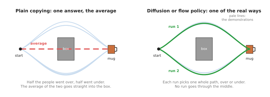
The left picture shows the problem, because the red dashed line is the average of the pale demonstrations, and it runs into the box. But the right picture shows what a diffusion policy does instead, which is that each time it runs it picks one whole path that looks like a real demonstration.
A task with more than one good way to do it is called multi-modal, and a mode is one of those good ways, so going left is one mode and going right is another. Diffusion policies were built to handle multi-modal tasks, because they learn the whole spread of ways that people did the task, and each time they run they pick one of them.
A flow policy does the same job with a method called flow matching, and it usually needs fewer clean-up steps, so it runs faster. Section 4 explains where that difference comes from.
2. What goes in and what comes out#
Section 1 said that the policy starts from a random guess, so that random guess is one of its inputs. So a diffusion policy for a robot arm takes in three things altogether.
- The latest camera pictures. Often there is one camera looking at the table and one camera on the wrist of the arm. Some policies take the last two or three pictures, so that they can see which way things are moving.
- The arm's own state. This is the angle of each joint and how open the gripper is, and the arm's own sensors measure these numbers.
- Some random numbers. This is the starting guess that gets cleaned up, and it is called noise, because it is random and has no meaning yet.
Then it gives back a chunk of actions, which is a short list of the next movements, one after another, such as the next sixteen positions for the gripper. The action chunking page explains why a chunk works better than one action at a time, and diffusion policies use chunks for the same reasons.
The table below turns that list into one concrete example. Read each row as one kind of input or output, with what it looks like for an arm picking up a mug.
| What it is | An example for picking up a mug | |
|---|---|---|
| In | camera pictures | one picture from above the table, one from the wrist |
| In | arm state | six joint angles and the gripper width |
| In | noise | a list of random numbers, the same size as the output |
| Out | an action chunk | the next sixteen gripper positions, each with "open" or "closed" |
3. How it works inside#
Section 2 listed the noise as an input, and this section follows what happens to it. The cleaning-up happens in steps, and each step uses the same neural network. A neural network is a large calculation with many adjustable numbers, which a computer tunes by showing it examples. Chapter 1 explains this in inside a neural network.
Here is what happens each time the policy is asked for a new chunk.
- The policy looks at the camera pictures and the arm state, and a part of the network turns them into a list of numbers that describes the scene.
- The policy makes a random chunk, where every position in it is random, so the chunk starts as a messy scatter of points.
- The network looks at three things, which are the scene description, the messy chunk, and how many clean-up steps are left. From those it works out which way each point should move to look more like a real movement.
- The policy moves each point a little way in that direction.
- Steps 3 and 4 repeat, and after the last step the chunk is a clean, smooth path.
- The arm plays the first part of the chunk, and then the policy looks again and makes a new chunk.
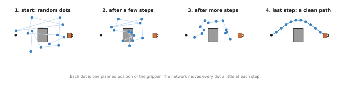
The picture shows one chunk being cleaned up. At the start the dots are random. Then at each step every dot moves a little, so by the last step they form a path from the start, round the box, to the mug.
But why does this whole procedure avoid the average? The answer is in step 2, because the random start is different each time. If the random dots happen to lean a little towards the top, then the clean-up pulls them into the "go over" path. But if they lean towards the bottom, the clean-up pulls them into the "go under" path. The network has learned where real paths are, rather than a single answer. So the random start decides which real path you get, and you never get the impossible middle.
The last step in the list, playing only part of the chunk, matters on a real robot. This is because the world can change while the arm moves, since a mug can be nudged. So the policy plays a few movements, looks again, and plans again. This is sometimes called receding horizon, because the plan always reaches a fixed distance ahead of where the arm is now.
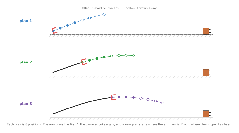
In the picture, each row is one plan of eight positions. The arm plays the four filled positions, throws away the four hollow ones, and starts a new plan from where it now is.
The six steps above are Diffusion Policy, which section 6.1 recommends as the model to train on your own recordings, and every other model in section 6 is a variation on them. What differs most between those models is how many times steps 3 and 4 repeat: 100 times for Diffusion Policy, 10 times for π0, π0.5 and SmolVLA, and 4 times for GR00T N1.7. Section 4 explains why some of them need so few. Those pretrained models, which are π0, π0.5, SmolVLA and GR00T N1.7, also read one input that the list above does not have, which is a sentence saying which task to do, and it joins the scene description made in step 1.
4. Diffusion and flow matching: the difference#
Section 3 described the clean-up steps without saying how the network learned to take them, and there are two ways to do that. Diffusion and flow matching both turn noise into a good chunk, but they differ in how the network learns the way from noise to the answer.
In diffusion, the network learns to remove a little noise at a time. This is an idea that came from models that make pictures, because those models learn to turn a screen of random coloured dots into a photo. So a diffusion policy does the same thing with a list of arm positions instead of a picture. But the path from noise to answer is wiggly, so it usually takes many small steps.
Instead, in flow matching, the network learns a direction to travel from the noise to the answer. During training, the method connects each noise sample to a real chunk by a straight line, and the network learns to point along those lines. Because the lines are straight, the policy can take a few big steps instead of many small ones.
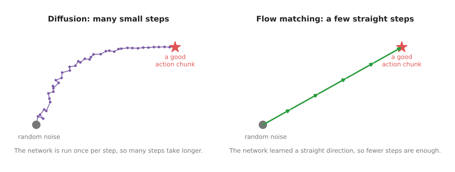
The left picture shows the many small, wobbly steps of diffusion. The right picture shows the few straight steps of flow matching, which end at the same kind of answer in less time.
Speed matters here because the network runs once per step. So if a policy needs many steps and each takes a few thousandths of a second, then the arm waits. Fewer steps means the arm can get a new chunk more often. This is one main reason most large robot models built in 2025 and 2026 use flow matching for their actions.
The table below compares the two methods, and you read across each row.
| Diffusion | Flow matching | |
|---|---|---|
| What the network learns | how to remove a little noise | which direction to travel |
| Shape of the way from noise to answer | wiggly | close to a straight line |
| Clean-up steps needed | many | few |
| Handles several good ways to do a task | yes | yes |
| Where you meet it | Diffusion Policy and Octo, in sections 6.1 and 6.5 | π0, π0.5, SmolVLA and GR00T N1.7, in sections 6.2 to 6.4, and most newer large robot models |
5. How it is trained#
Sections 3 and 4 described a network that already knows where real paths are, and this section says how it learned that. A diffusion policy learns from demonstrations, where a demonstration is one recording of a person doing the task by driving the robot. The recording keeps the camera pictures, the joint angles, and the commands the person gave, all at the same moments. Chapter 1 explains where such recordings come from, in where the data comes from.
So training a diffusion policy works in the six steps below.
- Take a short piece of one demonstration, which is the pictures at one moment and the next sixteen actions the person really took.
- Add a known amount of random noise to those sixteen actions, so that they become messy.
- Ask the network which way the messy actions should move to get back to the real ones.
- Compare its answer with the right answer, which you know, because you added the noise yourself.
- Adjust the network's numbers a little, so that the next answer is closer.
- Repeat with many pieces and many different amounts of noise.
Flow matching training is almost the same, and the difference is in step 3. There the network is asked for the straight-line direction from the noise to the real actions.
So how much recorded data does a diffusion policy need? For one task, such as "put the mug on the plate", people usually record somewhere between tens and a few hundred demonstrations. Large general models that do many tasks are trained on far more, pooled from many robots, and then adjusted to a new task with a smaller set, and the vision-language-action page covers those.
In every case, training needs a computer with a graphics card. A graphics card, or graphics processing unit (GPU), is a chip that does many small sums at once, which is what training a network mostly is.
6. Well-known models of this kind#
Section 5 described the training that all of these models share, and this section names the ones you can download and run. For each model it says what it is, why you would pick it rather than the obvious alternative, what it costs you, and which library runs it.
Read the table as a shortlist, with one row per model. The left column names the
model and says how much use it gets. The right column holds the rest: what it is best
at, its size, how many steps it takes per chunk, the memory it needs to train, the
licence on its code and on its weights, and when to pick it. Steps per chunk is how
many times the network runs to produce one chunk of actions, which section 4 said is
what decides the speed, and every such figure is the default in
LeRobot's own configuration file for that
policy. Do not read those step counts as a speed ratio on their own, because the
networks differ in size, and section 6.1 sets that out. The memory figures are the
video memory LeRobot's hardware guide gives for training at batch size 8. A cell says
not stated where the project publishes no number, because a guessed number is worse
than none.
| Model | What decides it |
|---|---|
| Diffusion Policy, most used in 2026 | It is best at one task, trained from your own recordings. Its size is not stated, and it runs the network 100 times for each chunk, which is the most of any row here. Training it needs about 8 to 14 GB. Its code is MIT, and you train the weights yourself. Pick it when you have one task, a few hundred demonstrations and one consumer graphics card. |
| π0 and π0.5, most used in 2026 among flow policies | They are best at being a pretrained policy that you aim at a new task with words. Their size is not stated, and they run the network 10 times for each chunk. Training them needs about 24 to 40 GB. Their code is Apache-2.0, and their weights are mixed, which section 6.2 sets out. Pick them when you have a large NVIDIA card and want pretraining and language instructions. |
| SmolVLA, most used in 2026 on cheap hardware | It is best at learning on cheap hardware. It has 450 million parameters, and it runs the network 10 times for each chunk. Training it needs about 10 to 16 GB. Both its code and its weights are Apache-2.0. Pick it when you work on a laptop or a Mac, or when you need one clean licence. |
| GR00T N1.7, worth betting on | It is best at being a pretrained policy with a vendor behind it. It has 3 billion parameters, and it runs the network 4 times for each chunk, which is the fewest of any row here. Training it needs about 24 to 40 GB. Its code is Apache-2.0, and its weights carry the NVIDIA Open Model License. Pick it when you have an NVIDIA card with 40 GB or more and want supported software. |
| Octo, historical | It is best at explaining where this design came from. Its size, its steps per chunk and the memory it needs to train are all not stated. Both its code and its weights are MIT. Never pick it for new work. |
6.1 Diffusion Policy, the one you train yourself#
Most used in 2026 for a single task, because it is the only model on this page that one person can train from nothing on one consumer graphics card.
Size not stated, a big card to train it on, MIT for the code, and the weights are yours because you are the one who makes them.
Diffusion Policy was published in 2023 by researchers at Columbia University, the Toyota Research Institute and the Massachusetts Institute of Technology, in the paper Diffusion Policy: Visuomotor Policy Learning via Action Diffusion. It is the model that made the method popular for robot arms, and it works exactly as section 3 described: camera pictures and arm state go in, and a chunk of actions comes out of the clean-up procedure. There are no general pretrained weights to download, so you train it on your own recordings.
The one idea it is built on is that the network never gives you a movement. It gives you a correction. You hand it a messy chunk, and it tells you which way every number in that chunk should move to look a little more like something a person really did, and then you hand it the result and ask again. The action chunking transformer on the page before this one does the opposite, because its pictures go in, its chunk comes out of a single pass, and it never sees its own answer.
That changes which parts sit inside the model and how often each one runs. There are two. A picture encoder reads the cameras and the joint angles and turns them into a short description of the scene, and it runs once for each decision. A correction network then runs over the chunk once for every clean-up step, and each time it is given three things, which are that scene description, the chunk as it stands, and how many steps are left. The paper is deliberate about keeping the pictures out of the clean-up. They are something the correction network is told about, and they are never made messy and cleaned up alongside the actions. That is why the cameras are read once for a decision rather than once for every step. The correction network itself comes in two shapes. One is a convolution that slides along the chunk from its first position to its last, so each correction is worked out from its neighbours in time. The other is a transformer that treats each messy position as a token. Its authors report that the convolution is easier to get working but smooths over sharp movements, while the transformer handles a sudden change of direction better and is fussier about its settings. LeRobot uses the convolution by default.
What the idea buys is the thing section 1 promised, plus one more. Two good routes
stay two routes, because the start is random and the corrections only push towards
places where real movements were. And the whole chunk is corrected together, so the
positions inside it agree with each other instead of being produced one at a time.
What it costs is that one decision is many runs of the network instead of one, and
that the clean-up schedule becomes another thing to set. You can buy most of that time
back in one line, by setting num_inference_steps lower and the scheduler to DDIM,
which is the noise schedule built to be skipped through, and you pay for it with a
slightly rougher path. Do not read the step counts in the table as a speed ratio,
though, because a step here runs a small network, while a step of π0 runs its action
expert over all the tokens its large pretrained half produced. Only a measurement on
your own machine settles which is quicker.
On a real arm the difference shows up in the recordings rather than in the code. The whole advantage of this policy over an action chunking transformer is that it keeps two ways of doing a task apart instead of averaging them, and it can only do that if both ways are in your data. If you always reach round the box on the left, you have paid for a hundred network passes and learned one route, and the transformer would have given you that same route in one pass. So recording for a diffusion policy means deliberately showing the alternatives, which is the opposite of what people do when they want tidy data.
The obvious alternative is π0 in the next sub-section, and the choice between them is the main decision on this page. Pick Diffusion Policy when your robot does one job. It is small, it needs no pretraining, nothing in it has to be fine-tuned, and you can look at every setting it has. Pick a pi model instead when you need the policy to follow an instruction in words, or when you have too few demonstrations to train from nothing.
The library is LeRobot, and it needs the diffusers package as well, because it
borrows the noise schedules from there. Install both with
pip install "lerobot[diffusion]". Building the policy takes a few lines more than
other policies, because you have to tell it the shape of your data first.
from lerobot.configs import FeatureType
from lerobot.datasets import LeRobotDatasetMetadata
from lerobot.policies.diffusion import DiffusionConfig, DiffusionPolicy
from lerobot.utils.feature_utils import dataset_to_policy_features

meta = LeRobotDatasetMetadata("lerobot/pusht")
features = dataset_to_policy_features(meta.features)
outputs = {k: f for k, f in features.items() if f.type is FeatureType.ACTION}
inputs = {k: f for k, f in features.items() if k not in outputs}

config = DiffusionConfig(
    input_features=inputs, output_features=outputs,
    horizon=64,                  # actions produced in one pass
    n_action_steps=32,           # of those, how many the robot carries out
    num_train_timesteps=100,     # clean-up steps used while training
    num_inference_steps=10,      # clean-up steps used while running: the speed dial
    noise_scheduler_type="DDIM", # DDIM allows fewer steps than the default DDPM
)
policy = DiffusionPolicy(config)
LeRobot gives you the network, the schedules, the training loop and the queue of
actions, and dataset_to_policy_features saves you from writing out the shape of
every camera and every joint by hand. Training is then one command with
--policy.type=diffusion. What you have to supply is the demonstrations, recorded in
LeRobot's dataset format with the alternatives in them. lerobot/pusht above is a
simulated pushing task with one camera and a two-number action, so it loads in
minutes and is a fair way to check that your installation works, but it is not a
robot arm.
One variant is worth knowing by name. 3D Diffusion Policy, or DP3 (2024) is the same method with a point cloud as its input instead of flat pictures, where a point cloud is a list of 3D dots on the surfaces a depth camera sees. The point cloud models page explains that input.
6.2 π0 and π0.5, the flow policies you can download#
Most used in 2026 among flow policies, because they are the only weights from a frontier laboratory that anybody outside the company can download.
Size not stated, a big card to run and a workstation to fine-tune, Apache-2.0 for the code, and a weights licence that depends on which copy you download.
π0, said "pi zero", was announced by Physical Intelligence on 31 October 2024 and opened on 4 February 2025. π0.5 followed on 22 April 2025 and added what its authors call open-world generalisation, meaning it also works in rooms it has never seen. The base checkpoints were trained on what the openpi repository calls 10,000 or more hours of robot data.
The one idea both are built on is that the hard part of a robot policy is understanding the scene and the instruction, and that somebody has already paid for that. So the part of a pi model that reads the pictures is not a small encoder trained on your own recordings, as Diffusion Policy's is. It is a pretrained vision-language model, PaliGemma in π0's case, which learned about pictures and words from the internet rather than from robots. The word "plate" in your instruction means something to it before it has ever seen a robot.
The clean-up is then done by a second, much smaller network, which the papers call the action expert, and the two are kept apart on purpose. The picture and word tokens go through the large pretrained half, the arm's state and the messy actions go through the action expert, and the only place the two meet is a shared attention step in which the action tokens may look at the picture and word tokens but not the other way round. The papers call this arrangement a mixture of two experts. One consequence matters every time the arm asks for a chunk: because the picture and word tokens never look back at the action tokens, their share of the work is done once for a decision, and only the small half repeats for each clean-up step.
That arrangement is also why the clean-up here is flow matching rather than the noise removal of Diffusion Policy. A clean-up step in a pi model is cheaper than running the whole model, but it is still far more work than a step of Diffusion Policy, because the action expert looks across every token the pretrained half produced. A hundred such steps for one decision would not be practical. The straight path from noise to the answer, which section 4 described and which needs only a handful of steps, is what makes bolting a clean-up network onto a large pretrained model usable at all.
π0.5 keeps both halves and adds a step above them. Before it moves, it writes the next subtask down in words, such as picking up the plate, and the action expert then produces the movements for that subtask rather than for the whole instruction. Its training ran in two stages too: in the first, the actions were turned into discrete tokens, like words, so that the whole model could be trained as plain next-word prediction, and the flow-matching half was added only in the second. The difference shows on a long job. Told to clear a table, π0 has to carry the decision about what comes next inside the same numbers that produce the movement, while π0.5 says "pick up the plate" first and then has only that movement to make. Its authors credit the breadth of π0.5 to training on many kinds of data together, which is web pictures and text, other robots, and those written-down subtasks, rather than to the extra step alone.
Pick one of these rather than Diffusion Policy when you want the pretraining. You can tell a pi model what to do in words, and because it has already seen a great deal of robot data, a new task needs fewer of your own demonstrations. The honest counterpart to that is a 2026 study called MINERVA, which found that flow matching gave no measurable advantage on its benchmarks over plain regression, meaning a policy that predicts the actions directly instead of cleaning up noise, while running several times more slowly. So the pretraining is the reason to choose a pi model, and the flow matching inside it is not by itself a reason.
Two of their costs have nothing to do with size, and both catch people. The openpi repository says it has only been tested on Ubuntu 22.04 and needs an NVIDIA card, so there is no usable path on a Mac. And the licence follows the exact file you download. openpi's code is Apache-2.0, its own checkpoints are served from the project's storage bucket with no separate terms named for them, the LeRobot copy at lerobot/pi0 declares Apache-2.0 on its model card, and the LeRobot copy at lerobot/pi05_base declares the Gemma licence, because of the language model inside it. Read the card of the exact checkpoint you download before you build anything you intend to sell.
The library is LeRobot again, which carries both as the pi0 and pi05 policy
types.
import torch
from lerobot.policies.factory import make_pre_post_processors
from lerobot.policies.pi0.modeling_pi0 import PI0Policy

model_id = "lerobot/pi0"
device = torch.device("cuda")      # this policy has no usable path on a Mac
policy = PI0Policy.from_pretrained(model_id).to(device).eval()

# Flow-matching steps per chunk. Ten is LeRobot's default for this policy,
# against the 100 of Diffusion Policy above.
policy.config.num_inference_steps = 10

preprocess, postprocess = make_pre_post_processors(
    policy.config, model_id,
    preprocessor_overrides={"device_processor": {"device": str(device)}},
)

with torch.inference_mode():
    action = postprocess(policy.select_action(preprocess(observation)))
LeRobot gives you the checkpoint, the normalisation that the model was trained with,
and the queue that hands out the 50 actions of a chunk one at a time. What you have
to supply is observation, which is one frame holding your camera pictures, your
arm state and the task written as a string, with the camera names the checkpoint
expects. For your own robot you then fine-tune, because a base checkpoint has never
seen your arm, and the
fine-tuning page
explains how much data and memory that takes.
6.3 SmolVLA, the flow policy that runs on a laptop#
Most used in 2026 by people learning on cheap hardware, because its authors say it runs on a MacBook and no other model here does.
Size m, a laptop to run it and a big card to train it, Apache-2.0 for the code and for the weights.
SmolVLA was released on 3 June 2025 by Hugging Face. It joins a SmolVLM2 vision-language backbone to a flow-matching action expert, and it was trained on about 10 million frames from 487 datasets contributed by the LeRobot community. Its authors report about 78 per cent success on real tasks with the SO-100 arm.
The one idea is not a new mechanism. SmolVLA has the same two halves as π0, a pretrained vision-language model and a small flow-matching action expert, and its authors set out to find how much of each half could be cut away before the policy stopped working. So the interesting part of this model is the list of corners it decided could be cut.
There are three, and all of them are about how much work one decision is. The first is that only the first half of the language model's layers are used at all, and the rest are never run, which its authors report as a good trade between speed and accuracy. The second is that each camera frame becomes only a few dozen tokens instead of a few hundred, by passing one whole picture rather than cutting it into tiles and by folding neighbouring pixels together. Fewer tokens is the cut that matters most for the action expert, because, as section 6.2 explained, the expert looks across all of those tokens on every clean-up step. The third is that the action expert alternates two kinds of layer, one that reads the vision-language half and one that only looks at the chunk itself. Its authors report that alternating the two did better than using either kind alone, both on success and on speed.
One more part of the release matters, and it is not a change to the model at all. It comes with an asynchronous runner, which lets the arm keep playing the actions it already holds while the next chunk is being computed, instead of standing still until the policy answers. That runner is part of LeRobot, so other policies can use it, but it is presented as part of this model's recipe, because a small model on a laptop is exactly the case where the wait is long enough to see.
Where the difference shows on a real arm is in what the model has already seen. The pi models were trained on a fleet of research robots that you do not own. SmolVLA's training frames were contributed by the LeRobot community, so much of that data was recorded on the same cheap arms a reader of this page is likely to have, which is why its reported numbers are on an SO-100 rather than on a laboratory platform. If your arm is an SO-100 and your computer is a MacBook, π0.5 will not run for you at all, and the model that has already seen arms like yours starts closer to your task.
Pick it rather than π0.5 for two reasons. It runs where π0.5 does not, including on a processor alone, and its code and its weights are both Apache-2.0, so there is no licence question to resolve before you ship. Against that, it is much smaller than a frontier model, so expect less of it, and its training data came from volunteers and is of uneven quality. What most often goes wrong is expecting frontier behaviour from a small model, and then blaming the recordings for it.
The library is LeRobot, installed with pip install "lerobot[smolvla]". The code
below is the pattern from the model's own card.
import torch
from lerobot.policies.factory import make_pre_post_processors
from lerobot.policies.smolvla.modeling_smolvla import SmolVLAPolicy

model_id = "lerobot/smolvla_base"
device = torch.device("mps" if torch.backends.mps.is_available() else "cpu")
policy = SmolVLAPolicy.from_pretrained(model_id).to(device).eval()

preprocess, postprocess = make_pre_post_processors(
    policy.config, model_id,
    preprocessor_overrides={"device_processor": {"device": str(device)}},
)

with torch.inference_mode():
    action = postprocess(policy.select_action(preprocess(observation)))
Only the class, the checkpoint name and the device differ from the pi code above,
which is the point of using one library for all of them. mps is PyTorch's name for
the graphics hardware in an Apple Silicon Mac. You still supply the same frame of
camera pictures, arm state and instruction, and your own demonstrations for
fine-tuning, because this is a base model rather than a finished one.
6.4 GR00T N1.7, the flow policy with a vendor behind it#
Worth betting on, because it is the clearest released evidence for the direction the field is taking, which is pretraining on ordinary human video, and because NVIDIA publishes it as a supported release rather than as a research drop.
Size l, a big card to run it and a workstation to fine-tune it, Apache-2.0 for the code and the NVIDIA Open Model License for the weights.
GR00T N1.7 was tagged on 18 April 2026 as a general-availability release, which NVIDIA defines as carrying support and stability guarantees.
The one idea it is built on is a change to what an action means. In Diffusion Policy and in the pi models, an action is normally an absolute target, which is where the gripper should be or what angle each joint should hold. In GR00T an action is a change from where the gripper is now, so "three centimetres to the left" is the action rather than a target coordinate. That sounds like a detail, and it is the whole reason the model exists in this form, because three centimetres to the left means the same thing on a human hand as on a gripper, while a target coordinate does not. So ordinary video of people doing things with their hands becomes training data, and the project says it pretrained on 20,000 hours of it alongside robot demonstrations.
Inside, it is the same two halves one more time, with two differences from π0.5. The vision-language half is Cosmos-Reason2-2B, a model built to reason about physical scenes rather than to describe pictures. The action half is a flow-matching diffusion transformer whose depth was halved, from 32 layers to 16, so the part that repeats on every clean-up step is cheaper than it would otherwise be. The table gives the other half of that saving, which is that GR00T asks for the fewest steps per chunk of anything on this page. One more thing follows from a single checkpoint driving several different bodies: it has to be told which body it is driving, through what the code calls an embodiment tag, and an arm it has never met is declared as a new one.
What the idea buys is pretraining data that nobody had to collect with a robot, which is a different bet from π0.5. π0.5 got its breadth from the web pictures and text its backbone had already read, plus a large fleet of real robots. GR00T is betting that human video, of which there is far more than there will ever be robot data, can carry the same weight. What it costs you is that the relative action space has to be switched on and configured, and that not every part of the arm can use it. The gripper stays absolute in the command below, because open and closed are not relative to anything.
The difference shows up on an arm that is not mounted where the demonstrated one was. An action that names a coordinate is only correct for one arrangement of arm, table and base, so moving the arm or putting it on a mobile base invalidates it. An action that says how far to move does not depend on that arrangement, which is why NVIDIA aims this model at humanoids, where the arm's own base moves as the robot walks.
Pick it rather than π0.5 when you want software somebody supports and a licence somebody has written down, since Physical Intelligence serves its checkpoints with no separate terms named for them. Pick π0.5 instead if you cannot accept NVIDIA's terms, or if your work is two-armed tabletop manipulation rather than the humanoid work GR00T targets.
Two more costs have nothing to do with size. The supported platforms are CUDA 12.8 desktop cards, Jetson Thor and Orin, and DGX Spark, so nothing about it runs on a Mac. And one sentence in the repository's README calls the model "fully commercially licensable under Apache 2.0", which is wrong about the weights: those are under the NVIDIA Open Model License Agreement, which allows commercial use but adds an attribution notice when you redistribute, a clause that ends the licence if you disable a safety guardrail without putting a similar one in its place, and a requirement to stay within NVIDIA's separately published terms. The licence section further down the README and the model card both say the narrower thing, and that is what misleads people here most often.
LeRobot carries it as the groot policy type, installed with
pip install "lerobot[groot]". Fine-tuning it on your own recordings is one command.
lerobot-train \
  --dataset.repo_id=$YOUR_DATASET \
  --policy.type=groot \
  --policy.device=cuda \
  --policy.base_model_path=nvidia/GR00T-N1.7-3B \
  --policy.embodiment_tag=new_embodiment \
  --policy.chunk_size=16 \
  --policy.n_action_steps=16 \
  --policy.use_relative_actions=true \
  --policy.relative_exclude_joints='["gripper"]'
LeRobot downloads the base model, converts your dataset into what GR00T expects and
runs the training. What you supply is $YOUR_DATASET, your own recordings in
LeRobot's format. new_embodiment tells it that your arm is not one of the bodies
the checkpoint already knows, and use_relative_actions turns on the relative action
space described above, while the gripper stays absolute.
6.5 Octo, kept for what it explains#
Historical. Size not stated, and the machine it needs is not stated either. MIT for the code and for the weights, which is the cleanest licence on this page.
Octo (2024) was an early open general policy trained on many robots' recordings, and it produced its actions with a small diffusion part at the end of a large transformer.
The one idea it is built on is that nothing should be built in. Everything that goes into the model becomes a token, the middle is a plain transformer, and every piece that belongs to one particular robot lives at the edges, so a new camera, a new instruction or a new arm is attached without re-initialising the trained middle. That is the opposite of a pi model, where the middle is one particular pretrained vision-language model and the shape of what you may feed it is settled by that choice.
Two parts of the arrangement are worth knowing because they are what makes the edges detachable. Pictures are cut into small patches and each patch becomes a token, an instruction goes through its own pretrained text encoder and becomes more tokens, and the transformer mixes whichever tokens are present, so a missing camera is simply missing tokens rather than a changed network. Then there is the readout token, which is an extra token allowed to look at everything before it while nothing is allowed to look at it. The small diffusion part reads the transformer through that token, so attaching a second head changes nothing about what the transformer computes.
The contrast with every model above it is where the understanding came from. Octo's transformer learned from robot recordings and nothing else, apart from the text encoder that reads the instruction, so whatever it knows about mugs and plates it learned from robots. π0, SmolVLA and GR00T all start from a model that read the internet first, and that single step is what the field did after Octo. The shape, which is a big model that understands the scene with a small generative head that produces the numbers, is still the shape every model above uses, and that is why Octo is worth reading.
Do not start new work on it. Its repository has had no commits since the middle of 2024, and LeRobot does not carry it, so you would be maintaining it yourself. Use SmolVLA for the same idea in supported code.
6.6 How to choose#
Start with Diffusion Policy inside LeRobot, trained on your own recordings, because one task on one consumer graphics card is the situation most readers of this page are in, and it is the only option here that does not depend on somebody else's checkpoint.
Four things change that answer.
If the robot has to be told what to do in words, or if you can only record a few dozen demonstrations, you need a pretrained policy instead. Choose SmolVLA when your computer is a laptop or a Mac, π0.5 when you have a large NVIDIA card and want the only weights a frontier laboratory has released, and GR00T N1.7 when you want a written licence and a vendor's support.
If the policy is too slow in your control loop, do not change model first. Set
num_inference_steps to 10 with the DDIM schedule, as section 6.1 showed, and
measure again.
If the task needs two arms working together, look at RDT-1B from Tsinghua University, a diffusion model built for that case, which is MIT on both its code and its weights. The learned motion document lists it with every other downloadable policy and the licence of each.
If the motion must be identical on every run, none of these is the right answer.
7. Where this is going#
Section 6 described the models as they stand, and this section is about where the method is heading. Four kinds of statement appear below, and they carry very different weight. A demonstration is a recording of something working once, under conditions the publisher chose. A product announcement says that something can be downloaded or bought, so you can check it yourself. A research result is a measured number under a stated protocol. A projection is a claim about a date that has not arrived, and it is the weakest of the four. Where a sentence below is my own expectation rather than somebody's claim, it says so. Book 3's what is coming to robot arms applies the same four words to the whole field.
7.1 How it got here#
The idea has not changed since 2023, and the number of network runs per movement has fallen from a hundred to four. Diffusion Policy showed that a clean-up procedure borrowed from picture generation could drive a robot arm, and a hundred runs for every decision was the price of it. Everything since has been an attempt to pay less for the same thing. Flow matching replaced the wiggly path from noise to answer with a nearly straight one, which cut the hundred to about ten. The expensive half of the model was then lifted out of the loop, so that the pretrained vision-language part runs once for a decision while only the small action expert repeats. GR00T N1.7 now asks for four steps. That count is the thread running through the rest of this section.
7.2 Where it is used in industry today#
The checkable part of this method's industrial position is that the models are downloadable. GR00T N1.7 has been on the Hugging Face Hub since 25 February 2026, and NVIDIA put it into LeRobot on 6 July 2026. The π0 and π0.5 checkpoints are served from openpi, and SmolVLA from Hugging Face. Those three are product announcements, which is the strongest kind of evidence here.
One company has published a careful measurement of the method at scale. Toyota Research Institute built what it calls Large Behavior Models by extending the Diffusion Policy design across a body of simulated and real robot data, and it measured them in blind, randomised trials against single-task policies ( project page). It reports that training on many tasks first made the policies both more successful and more robust, and let a hard new task be taught from a fraction of the data a single-task policy needed. That is a research result and not a product, because nothing from it is downloadable. Its value here is that the protocol was built to stop its own authors fooling themselves, which is unusual in this area.
What is missing is the kind of fact any industrial automation vendor publishes as a matter of course. Nobody has said how many robots run one of these policies at a named customer site, for how many hours, or how often a person had to step in, and Book 3's frontier chapter finds the same gap across the whole field in its section on what is promised that the evidence does not support. So read the deployment videos as demonstrations. What is established is narrower and still worth knowing, which is that this method is how almost every downloadable policy now produces its actions.
7.3 What is being worked on right now#
The live problem is the one section 4 introduced. A control loop has a time budget, the network runs once per clean-up step, and so the number of runs per movement decides whether a policy fits the loop at all. Three lines of work attack that number, and they do not conflict, so one policy can take all three.
The first is to take fewer steps, by compressing a policy you have already trained. Consistency Policy distils a trained Diffusion Policy into a faster one, by making the student agree with itself along the paths the teacher learned. Its authors report inference an order of magnitude faster than the quickest alternative they compared against, with competitive success rates on six simulated and three real tasks, running on a laptop graphics card, and they report that the procedure is not fussy about how good the teacher was. That is a research result. The appeal for a reader of this page is that you keep the policy you trained on your own recordings and pay once to compress it, instead of changing model.
The second is not to wait for the answer at all. Real-time chunking, published by Physical Intelligence in June 2025, computes the next chunk while the arm is still playing the current one. It freezes the actions that are certain to be carried out and fills in the rest around them, which is what stops the join between two chunks being a pause or a jerk. Its authors report that it works on any diffusion or flow policy with no retraining, and they measure it on twelve simulated tasks and six real two-armed ones, including lighting a match, with delay deliberately added. That is a research result. The same idea is shipped code rather than a paper in LeRobot's asynchronous inference, which section 6.3 mentioned as part of SmolVLA's release, and that is a product announcement.
The third is to make each step cheaper by making the model smaller. FoldQuantVLA reports four-bit weights and four-bit activations with speed-ups of 1.20 to 1.33 times, where storing each number with fewer bits is called quantisation. The reason this corner is busy has nothing to do with research fashion. NVIDIA announced three new Jetson Thor computers on 15 July 2026, which are computers for running a model on the robot itself, with physical hardware stated for the first quarter of 2027, and the smallest of the three has 16 gigabytes of memory. Today's large policies do not comfortably fit in that. The announcement is dated and checkable, and it sets the size a policy has to be.
7.4 What is still unsolved#
The first unsolved thing is whether the clean-up earns its cost at all. Section 6.2 quoted MINERVA, which found no measurable advantage for flow matching over plain regression on its benchmarks while running several times more slowly. Nobody has published a measurement on a real arm showing that a diffusion or flow policy keeps two ways of doing a task apart better than a plainly trained policy of the same size does. The argument in section 1 is a good one, and it is still an argument rather than a number. Three years after the method arrived, that hole in the evidence is the most surprising thing on this page.
The second is that you cannot compare two policies' speed from anything published. The step counts in section 6 come from each project's own configuration file, and a step means a different amount of work in each row, as section 6.1 said. No project reports actions per second on named hardware with the camera resolution and the chunk length stated, so only a measurement on your own machine settles anything. IndustrialVLA-Bench proposes a shared reporting format for open policies, and whether anybody adopts it is not yet established.
The third is that a faster clean-up does not buy you hands. Google DeepMind's own post of 30 July 2026 on Gemini Robotics 2 says that while its models reach a medium to high success rate with grippers, "the multi-finger dexterous manipulation remains challenging". Book 3's frontier chapter says the same from the other side, because the share of robotics abstracts mentioning dexterity moved only from 3.64 per cent in 2025 to 4.16 per cent in 2026. A policy that answers in four network runs rather than a hundred still has to be told what to do with five fingers.
7.5 The next two to three years#
I expect running the policy and playing the actions at the same time to become ordinary, rather than a feature of one release. This is my expectation and not an announcement. The reason is that it is the cheapest of the three attacks in section 7.3. Real-time chunking needs no retraining and works on any policy of this kind, and LeRobot's runner already serves every policy that library carries, so taking it costs a change of configuration rather than a change of model. A speed-up that is both free and general stops being news and becomes the default.
I expect the number people quote to change, from clean-up steps per chunk to actions per second measured from camera to motor on named hardware. This is my expectation, and the reason is arithmetic. At four steps the clean-up is no longer where the time goes, so the step count has stopped being informative, and the size of the pretrained half, the camera resolution and the chunk length now decide the answer. The frontier chapter's measurement that the share of robotics abstracts mentioning a benchmark rose from 15.27 to 20.04 per cent in a year is the supporting evidence rather than my guess.
I expect the open default to become a policy sized for a 16 gigabyte computer on the robot. This one rests on a dated product announcement rather than on my judgement, which is why I would bet on it hardest. NVIDIA has stated hardware for the first quarter of 2027 whose entry-level part has 16 gigabytes, that part is what a small company or a university will buy, and a policy that does not fit the computer people buy loses to one that does, whichever is better. So quantisation and small backbones gain adoption for a reason that has nothing to do with whether they are interesting, and SmolVLA is the model on this page already closest to that shape.
I expect distilling your own trained policy into a few-step one to become a routine last stage, in the way that shrinking a language model already is. This is my expectation. The reason is that it suits the reader this page is written for. Section 6.1 recommends training Diffusion Policy on your own recordings, that is the model with a hundred steps, and Consistency Policy's authors report that the compression is cheap next to the training and tolerant of a mediocre teacher. The second reason is that waiting for a faster frontier model to be handed to you is a bet the record does not support, because Physical Intelligence has published no weights for π*0.6 or π0.7, and both are now past the three to five month gap its first two models set.
I expect flow matching to stay, and the claim made for it to get narrower. This is my expectation, and it is the one most likely to annoy people. It stays because it is what makes attaching a clean-up network to a large pretrained model affordable at all, which section 6.2 explained. The claim that narrows is the one about accuracy. After MINERVA, the honest reason to pick π0.5, SmolVLA or GR00T N1.7 is the pretraining inside it, and anybody selling you flow matching as more accurate than predicting the actions directly should be asked for the measurement. The shape itself, which is a large pretrained half that understands the scene and a small generative half that produces the numbers, has survived four generations of model, so I do not expect this family to be replaced inside the window.
8. Where to read next#
This page finishes the three copying policies, so the reading below either goes back over them or moves on to the methods that do not copy at all.
In this chapter:
- Behaviour cloning explains copying demonstrations, and the drifting problem that chunks help with.
- Action chunking transformers explains chunks in detail.
- Reinforcement learning policies is the next page, and it learns by trying and scoring, instead of by copying.
- The movement models overview compares every kind in this chapter.
In other chapters of this book:
- Vision-language-action models are large models that use flow matching inside them.
- Running a model on a robot explains why speed matters on a real arm.
Deeper documents elsewhere in this repository:
- Learned methods for one arm, behaviour cloning covers diffusion and flow matching in more detail, with evidence.
- Learned motion explains which part of an arm's movement a policy should and should not replace.