This page is about neural networks that read a point cloud directly, so it answers three questions. How can a model take in a list of 3D points that has no order, and what does it give back to a robot arm? And when is it better than turning the points into a picture and using an ordinary image model?
It is for a reader who has read the chapter overview, which explains what a point cloud is. You should also know, from inside a neural network, that a network is made of layers that turn a list of numbers into another list of numbers.
Before this page, it helps to have read clustering, which splits a point cloud into objects with written rules and thins it onto small cubes called voxels. This page shows what a trained model adds.
Contents#
- What it is
- What goes in and what comes out
- How it works inside
- How it is trained
- Well-known models · 5.1 PointNet · 5.2 PointNet++ · 5.3 MinkowskiEngine and spconv · 5.4 Point Transformer V3 · 5.5 Sonata · 5.6 How to choose
- Where this is going
- Where to read next
1. What it is#
Since the overview explained what a point cloud is, this section says what a model does with one. A point cloud model is a neural network that takes a list of 3D points and says what they are.
For example, imagine someone gives you a sheet of paper with 1,000 rows. Each row
has three numbers, which are the x, y and z of one spot on some object.
The rows are in a random order, and your job is to say whether the object is a mug,
a bottle or a book. A person would plot the dots first and then look at the shape.
But a point cloud model has to do the same job without plotting anything, because it
only has the numbers.
2. What goes in and what comes out#
The sheet of paper in the last section is close to what the model really gets. A
point cloud model takes in one point cloud, and each point in it has at least three
numbers, which are x, y and z. Some models also take the colour of each
point, as three more numbers for red, green and blue.
Before the cloud goes in, the software usually cuts it down to a fixed number of points, such as 1,024 or a few thousand. It does this by picking points spread evenly over the cloud, because a full depth camera shot has far more points than a model needs.
What comes out depends on the job, and there are two common jobs.
- Classification gives one name for the whole cloud, such as "mug", together with a number between 0 and 1 that says how sure the model is.
- Segmentation gives a name to every single point, so on a table scene each point is marked "mug", "box" or "table". On a single object, each point can be marked with a part name instead, such as "handle" or "body", and that is called part segmentation.
The picture below shows segmentation on a small table scene.
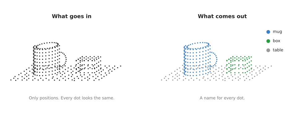
On the left the model sees only positions, so every dot looks the same. On the right every dot has a name, shown here as its colour.
For a robot arm, segmentation is usually the more useful of the two jobs. Once the arm knows which points are the mug, it can work out where the mug is, how big it is, and where to put its fingers.
3. How it works inside#
The random order of those rows is the first thing the design has to deal with, so this section starts there.
The problem of order#
An image model can rely on order, because pixel number 5 in a row is always next to pixel number 4 and pixel number 6. A point cloud has no such order, since the camera driver can list the points in any order it likes and it is still the same scene.
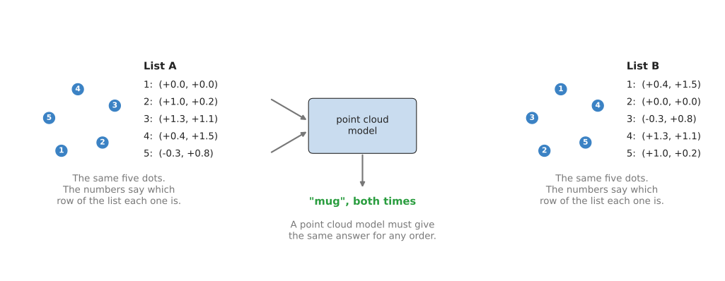
List A and list B hold the same five dots in a different order, and a point cloud model must give the same answer for both.
An ordinary network cannot do that, because it treats the first number in its input list differently from the second. So if you fed it list A and then list B, it would see two different inputs and could give two different answers. That means a point cloud model needs a design that ignores order altogether.
One small network for every point, then the largest number#
The first model that solved this well is called PointNet, and researchers at Stanford University published it in 2017. It is explained here because every later model on this page reuses its two ideas, and section 5.1 says why you should read it rather than run it. It works in four steps.
- Take one point, as its three numbers.
- Pass it through a small network, which turns those three numbers into a longer list of numbers. In the real PointNet this list has 1,024 numbers, while the picture uses four so that you can read them.
- Do the same for every other point, with the same small network, so that every point now has its own list of numbers.
- Look along each position in those lists and keep only the largest number, which is called max pooling. The result is one list for the whole cloud.
A last small network then turns that one list into the answer, such as "mug".
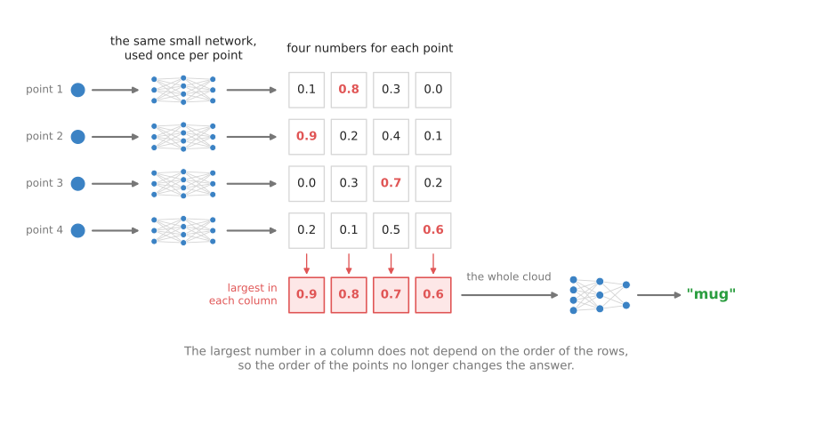
Each row is one point's list of numbers, and the red numbers are the largest in each column, which become the list for the whole cloud.
Step 4 is the step that removes order, because the largest number in a column is the same whichever row it sits in. So if you shuffle the points, the rows move but the red numbers stay the same.
Each number in the lists comes to stand for some small feature of shape. One number might come out large for points on a curved surface, while another might come out large for points far from the middle. Nobody chooses these features, because the network learns them during training. The largest value in a column then says that somewhere in this cloud there is a point with this feature.
For segmentation, PointNet goes one step further and sticks the list for the whole cloud onto each point's own list. Each point then knows about itself and about the whole shape, so a last small network can give each point its name.
Looking at neighbours#
PointNet has one weakness, which is that each point goes through the small network alone and never looks at the points right next to it. So PointNet is poor at small details, such as the thin gap between a handle and the side of a mug.
Instead, PointNet++, from the same group later in 2017, fixes this by looking at small groups of points first. Section 5.2 recommends it, and explains that you usually meet it inside a grasp model rather than calling it yourself.
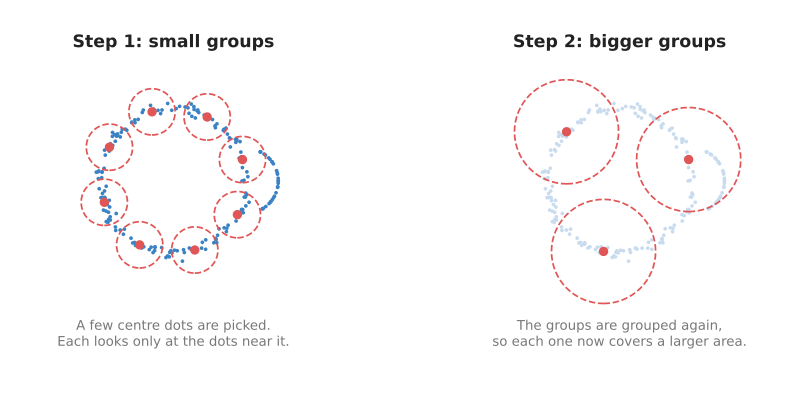
On the left, each red centre looks only at the dots inside its small circle, while on the right the groups are grouped again to cover a larger area.
It works in rounds, and in each round it does three things.
- Pick a number of centre points, spread out over the cloud.
- For each centre, collect the points within a small distance of it.
- Run a small PointNet on just that group, which gives one list of numbers for the whole group.
The next round then uses the centres of those groups as its points, with a bigger distance. So the model first learns the shape of small patches, then of larger parts, and then of the whole object. This is the same pattern that image models use when they look at small patches of pixels first. The seeing models chapter describes that pattern for pictures.
Two other ways in#
Besides PointNet and its neighbour groups, two other designs are common today.
The first cuts space into small cubes called voxels, where a voxel is simply a 3D pixel. The model marks each cube that has a point in it and then works on the grid of cubes. Most cubes in a room are empty air, so the model only computes on the cubes that hold points. That trick is called sparse convolution, and it is fast on large scenes. Section 5.3 recommends the two libraries that people run it with.
The second design uses attention, which is a way for each point to look at other points and decide which of them matter to it most. It is the same idea that language models use to decide which words in a sentence matter to each other. Point Transformer models use it on groups of nearby points. Section 5.4 recommends the current one, Point Transformer V3, which reaches its neighbours by sorting the points into an order rather than by searching for them.
4. How it is trained#
Whichever of those designs a model uses, it learns from point clouds that people have already labelled. For classification, each example is a whole cloud with one name, while for segmentation each example is a cloud with a name on every point. Most of that data comes from one of three places.
- Collections of 3D shapes made on a computer, such as ModelNet40 and ShapeNet, where ModelNet40 has about 12,000 shapes in 40 kinds such as chairs, cups and aeroplanes. Software then samples points from the surface of each shape to make a cloud.
- Scans of real rooms, such as ScanNet, which has more than a thousand scans of indoor rooms made with a depth camera, and people marked each part of each scan by hand.
- Simulation, where a robot team places 3D models of its own objects in a simulated bin and makes a simulated depth camera look at them. The simulator knows which object every point came from, so the labels cost nothing.
All three of those places need somebody to label the points first, and there is a fourth route that does not. A model can be trained on unlabelled clouds, by giving it a task whose answer is already in the cloud, and then it needs only a few labelled clouds of yours to finish the job. Section 5.5 recommends Sonata, which is a Point Transformer V3 trained that way.
Training itself works as in how a model learns. The model guesses the names first. Then the training program compares them with the right names and adjusts the network a little so that the next guess is closer. This whole loop repeats many thousands of times before the model is any good.
One more step in training makes a large difference to the result. The program turns each cloud by a random angle, moves it a little, and shakes each point by a small random amount. This teaches the model that a mug turned sideways is still a mug, and it also prepares the model for the noise a real depth camera adds.
5. Well-known models#
The designs above appear in real code under real names, and this section is the shortlist. It says what each one is best at, what it costs you, and what to type to run it.
Read the table as a first pass, then read the sub-section for the one or two you are considering. The left column names the model and says how current it is. The right column holds everything that decides between them: what the model is best at, how big the download is, what its licence allows, and when to pick it. Read the download part carefully, because several of these ship code with no trained weights at all, and a model with no weights is a model you have to train yourself. Every licence below was read from the project's own licence file.
| Model | What decides it |
|---|---|
| PointNet, historical | It gives one name to one object that has already been cut out of the scene. The download is code only, because no weights were released, and the licence is MIT. Pick it when you are learning how these models work. |
| PointNet++, most used in 2026 | It names one object and its parts, from a few thousand points. The download is code only, because no weights were released, and the licence is MIT. Pick it when the grasp model you want already contains it. |
| MinkowskiEngine and spconv, most used in 2026 | They carry whole rooms and full bins, of hundreds of thousands of points. What you download is a library rather than a model, under MIT for MinkowskiEngine and Apache-2.0 for spconv. Pick them when speed on a large cloud decides the job. |
| Point Transformer V3, most used in 2026 | It puts a name on every point of a room scan. The ScanNet checkpoint is 554 MB, and the code is MIT licensed. Pick it when accuracy on a whole scene matters most. |
| Sonata, worth betting on | It does the same job with far fewer labels of your own. The download is 434 MB, with about 108 million learned numbers, and the code is Apache-2.0 while the weights are CC BY-NC 4.0. Pick it when you have few labelled clouds and no product to ship. |
5.1 PointNet#
PointNet is historical, and it is on this list because every later model here reuses the two ideas in section 3.
Size xs, a laptop, MIT for the code, and no weights were released, so there is no weights licence to read.
Charles Qi and colleagues at Stanford University published it at the 2017 Computer Vision and Pattern Recognition conference, usually written CVPR. It is the one shared small network per point, followed by max pooling.
The one idea it is built on is that the answer must not change when somebody shuffles the rows of the input, and that the safe way to get that is to build the model out of steps which cannot see the order at all. The authors did not train the network to ignore the order of the points. They assembled it from parts to which the order is not available, so the guarantee comes from the shape of the model rather than from what it learned.
Inside, that leaves only two kinds of part. The first is a small network that reads one point, as three numbers, and writes a longer list of numbers for that point. The same network, with the same learned numbers, runs on every point separately, so it has no way of knowing which row it was handed. The second is the max pooling step, which reads all those lists and keeps the largest number in each column. What flows from the first part to the second is one list per point, and what leaves the second is a single list for the whole cloud. The published model has one more part that section 3 left out: a small side network that looks at the cloud and predicts a three-by-three table of numbers, which is then multiplied into every point to turn the whole cloud into a standard orientation before the main network sees it. Even so, the thing to take away is what is absent. Nowhere in PointNet is the distance between two points worked out, and no point is ever shown the numbers of another point. Every later model on this page adds exactly that, and the three designs that follow add it in three different ways.
What the idea buys is that the work is a straight line in the number of points. Each point costs one pass through a small network, nothing is compared against anything else, so there is no search to do and an ordinary processor keeps up. What it costs is that the single max pooling step is the only channel from one point to another. A column's largest number says that some point in the cloud had this feature strongly, and it cannot say which point, nor whether two features sat two centimetres apart or on opposite sides of the table. So PointNet ends up holding a list of the features an object has rather than an arrangement of them, and fine shape is exactly the information that an arrangement carries.
On a robot arm the difference shows up at the boundary between two parts of one object. Give PointNet a mug that has already been cut out of the scene and ask whether it is a mug or a bottle, and a list of features is enough, on the arm's own processor with no graphics card at all. Ask it instead which points are the handle and which are the side, and it has to answer for a point near the join using features that were pooled over the whole mug, so the boundary lands roughly in the right area rather than on the join. PointNet++ in the next sub-section is the first model here that can put it on the join, because there each point's answer is computed from the handful of points around it.
The obvious alternative is its own successor, PointNet++, and you should normally use that instead. There is one case for plain PointNet: it does no neighbour search at all, so it is the only model here that runs at a sensible speed on an ordinary processor with no graphics card, and on a single object already cut out of the scene it is often accurate enough.
What it costs you beyond that is the training and the install. No weights for everyday objects were released, so the labelled clouds and the training loop are yours, and the original repository will not run on a current install, since its own instructions say it was tested with Python 2.7, TensorFlow 1.0.1 and CUDA 8.0.
PyTorch Geometric supplies the pieces, as MLP for the small network and
global_max_pool for the pooling step.
import torch
from torch_geometric.nn import MLP, global_max_pool

pos = torch.rand(1024, 3)                      # one cloud of 1,024 points
batch = torch.zeros(1024, dtype=torch.long)    # every point belongs to cloud 0

# The same small network runs on every point on its own, turning each point's
# three numbers into 1,024 numbers.
per_point = MLP([3, 64, 64, 1024])(pos)

# Keep the largest number in each of those 1,024 columns. This is the step that
# makes the answer the same whatever order the points arrive in.
cloud = global_max_pool(per_point, batch)      # one row of 1,024 numbers

# A last small network turns that row into one score per object kind.
scores = MLP([1024, 512, 40], norm=None)(cloud)
The library gives you the layers and the pooling. You supply everything else: the
labelled clouds, the training loop, and the step that cuts each object out of the
scene before it reaches this code. The batch vector is not an optional detail,
because it is how PyTorch Geometric tells one cloud from another when you pass
several at once.
5.2 PointNet++#
PointNet++ is most used in 2026, although usually not by you directly, because it sits inside grasp models that you call instead.
Size xs, a small card, MIT for the code, and again no released weights.
The same Stanford group posted it in June 2017. It adds the rounds of neighbour grouping described in section 3, and each round picks centre points, collects the points near each centre, and runs a small PointNet on each group.
The one idea is to run PointNet many times on small groups of nearby points instead of once on the whole cloud, and then to run it again on what comes out. A group of points that all sit within a few centimetres of each other is small enough that pooling over it loses almost nothing, and the result of one round is a shorter cloud which the next round can treat as its input.
Inside, one round has three parts. The first picks the centres, by starting anywhere and then repeatedly adding the point that is furthest away from every centre picked so far, which spreads them over the cloud; the authors call this farthest point sampling. The second collects, for each centre, the points lying within a fixed distance of it in metres. The third runs a small PointNet on each group on its own. What comes out is a shorter cloud whose points are the centres, and whose features describe the neighbourhood around each centre instead of a single position. Two things are therefore different from PointNet, which did neither of them. Distances between points are now worked out, which is the work PointNet carefully avoided. And max pooling now happens many times over small groups rather than once over everything, so where a feature was found is no longer thrown away: it survives as the coordinates of the centre that found it. The paper adds one further part for the sake of real depth cameras, which is that a centre can look at two or three different distances at the same time and the results are joined, because a surface close to the camera gives many points per square centimetre while a far one gives very few.
What the idea buys is fine shape, and a sense of size measured in metres. A point near the join of a handle is now described by the points within a few centimetres of it, nearly all of which are also handle, so the boundary lands on the join. What it costs is first that same distance, which you have to choose: it is in metres, so a model trained on mugs does not transfer to pallets without being trained again, and a distance set too large smooths small objects away. The second cost is time that grows faster than the cloud does. Both the centre picking and the collecting compare points against other points, so doubling the number of points more than doubles the work, which is why people thin the cloud down first and why section 5.3 exists.
On a robot arm the gain over PointNet shows up in part segmentation, and the limit shows up in size. A few thousand points around one object is where PointNet++ is at its best, and a few thousand points around one object is exactly what a grasp model hands it. A whole work cell seen from two metres away is where it gives up: either the distance is small enough to see the objects and the rounds take too long, or it is large enough to be quick and the objects are too small to survive it. The next two sub-sections are the two ways out of that.
The obvious alternative is Point Transformer V3 in section 5.4, which is more accurate on scenes. Pick PointNet++ for two reasons. The first is that your input is one object rather than a room, and with a few thousand points grouping is cheap while the extra machinery of a transformer buys little. The second is practical: Contact-GraspNet and several other grasp models were built on PointNet++, so if you use one of them, as the six-DOF grasps page describes, you are already running it and the choice is made.
One other design from those years is worth recognising by name. DGCNN finds each point's neighbours again at every layer, in the space of learned features rather than in metres, which makes it good at naming the parts of a single object. Its repository last changed in 2022, so read about it rather than build on it.
What it costs you beyond that is that there is no package to install. There is no
pip install pointnet2, there are no released weights for your objects, and the
original repository needs TensorFlow 1.
PyTorch Geometric supplies the one round, which the PointNet++ paper calls set
abstraction, out of fps, radius and PointNetConv.
import torch
from torch_geometric.nn import MLP, PointNetConv, fps, radius

class SetAbstraction(torch.nn.Module):
    """One PointNet++ round: pick centres, group neighbours, run a PointNet."""

    def __init__(self, ratio, r, nn):
        super().__init__()
        self.ratio, self.r = ratio, r
        self.conv = PointNetConv(nn, add_self_loops=False)

    def forward(self, x, pos, batch):
        idx = fps(pos, batch, ratio=self.ratio)        # keep a fraction of the
                                                       # points, spread out
        row, col = radius(pos, pos[idx], self.r, batch, batch[idx],
                          max_num_neighbors=64)        # neighbours within r metres
        edge_index = torch.stack([col, row], dim=0)
        x_dst = None if x is None else x[idx]
        x = self.conv((x, x_dst), (pos, pos[idx]), edge_index)
        return x, pos[idx], batch[idx]                 # fewer points, richer features

# A first round over 20 cm neighbourhoods, keeping half the points.
layer = SetAbstraction(0.5, 0.2, MLP([3, 64, 64, 128]))
The library gives you the sampling, the neighbour search and the grouping. You supply the stack of rounds, the head that produces names, the training data, and the radius for each round. That radius is in metres, so it is the one number you must set from the real size of your objects.
5.3 MinkowskiEngine and spconv#
Sparse convolution is most used in 2026 whenever the cloud is a whole room or a full bin, and these two libraries are how people run it.
Size not stated, because what you download is a library and not a model, a big card, and MIT for MinkowskiEngine against Apache-2.0 for spconv.
Both do the same thing: they cut space into small cubes, called voxels, and do
convolution only on the cubes that contain points. MinkowskiEngine comes from Chris
Choy and NVIDIA, with its paper at CVPR 2019, and spconv is a separate library that
installs from pip in a build that matches your CUDA version. These are libraries
rather than single models, so you pick a network, such as the MinkUNet family, and
run it on top.
The one idea is to stop treating the points as a set and to give them a grid address instead. Round each point's three numbers to the nearest cube, keep only the cubes that caught at least one point, and the question "which cubes are next to this one" turns into arithmetic on the address rather than a search through the cloud.
Inside, the cloud is then held as two tables, and that shape is the thing worth
remembering. One table has a row per occupied cube holding its whole-number address,
and the other has a row per occupied cube holding that cube's features. A layer does
what an image convolution does: for each occupied cube it reads the few addresses
around it, multiplies what it finds there by the learned weights, and writes one row
of output. So the networks built this way are shaped like image networks, and MinkUNet
is a U-net, which halves the resolution a few times, climbs back up, and carries links
across from each level to the matching level on the way up. Against PointNet++, three
parts have simply disappeared. Farthest point sampling is gone, because halving the
resolution is division. The search for the points within a distance is gone, because
the neighbours are computed from the address. And max pooling is no longer what makes
the answer independent of order, since the rounding step now does that: two points
that land in the same cube become one row whichever of them arrived first. One choice
is left, and it decides whether a deep network is affordable: whether a layer may
write output in cubes that held no points. If it may, the occupied set widens a little
at every layer until the cloud is no longer sparse. If it may not, the layer copies the
occupied addresses to its output and computes only there, which spconv's documentation
sums up as the output keeping the same indices as the input, and spconv offers the two
as separate layers, SparseConv3d and SubMConv3d.
What the idea buys is a cost that follows the number of occupied cubes rather than the
number of points, and that is the whole reason a scan of a room fits on one card. A
single depth camera frame can hold three hundred thousand points and far fewer
occupied cubes, and the second number is the one you pay for. What it costs is that
the rounding happens before the network starts and cannot be undone. Anything thinner
than one cube is gone, and the answers come back one per cube rather than one per
point, so something has to carry them back to the points you started with, which is
what the slice call in the code below is for.
On a robot arm, the difference from PointNet++ shows up the first time you point the camera at the whole bin instead of at one object. Sparse convolution takes the bin in one pass and does not mind that the near surfaces are dense and the far ones thin, while PointNet++ would need the cloud thinned to a few thousand points first, and the thinning is where the small parts are lost. It goes the other way on a single mug with a three-millimetre handle: at two-centimetre cubes that handle is barely one cube wide, and PointNet++, which rounds nothing, is the better choice.
The obvious alternative is the neighbour grouping of PointNet++. Voxels win on large clouds because they make the neighbour question free: a cube knows which cubes are next to it from their addresses alone, so there is no distance search at all, while PointNet++ must search every time. That one difference is why sparse convolution carries scans of whole rooms and grouping does not.
What it costs you is the voxel size and the install. The voxel size is yours to choose and it sets the finest detail the network can ever see. The install is the usual place this goes wrong, because both libraries compile CUDA code against your exact PyTorch version. MinkowskiEngine's repository last changed in March 2024, so building it against a current PyTorch and CUDA is now the common failure, and the host that its own example downloads pretrained weights from no longer answers. spconv is the better-maintained of the two, and Point Transformer V3 in the next sub-section is built on it, so you may end up installing it anyway.
MinkowskiEngine's own examples/indoor.py names every point of an indoor scan with a
MinkUNet34C trained on ScanNet.
import numpy as np, open3d as o3d, torch
import MinkowskiEngine as ME
from examples.minkunet import MinkUNet34C

model = MinkUNet34C(3, 20).cuda().eval()      # 3 colour channels in, 20 names out
model.load_state_dict(torch.load("weights.pth"))

cloud = o3d.io.read_point_cloud("room.ply")
coords = np.asarray(cloud.points)
colors = torch.from_numpy(np.asarray(cloud.colors)).float() - 0.5

voxel_size = 0.02                             # 2 cm cubes, so 2 cm is the limit
field = ME.TensorField(
    features=colors,
    # Dividing by the voxel size turns metres into cube numbers.
    coordinates=ME.utils.batched_coordinates([coords / voxel_size],
                                             dtype=torch.float32),
    quantization_mode=ME.SparseTensorQuantizationMode.UNWEIGHTED_AVERAGE,
    device="cuda")

with torch.no_grad():
    out = model(field.sparse())               # one row per occupied cube
    names = out.slice(field).F.argmax(dim=1)  # back to one name per point
The library gives you the grouping of points into cubes, the convolution that skips
empty space, and the slice call that maps each cube's answer back onto the original
points. You supply the network and its weights, and because of the broken download
above you should expect to train on your own labelled scans. You also supply the 20
names, because this network was trained on ScanNet's furniture classes, such as wall,
floor, chair and table, which are not the objects on a workbench.
5.4 Point Transformer V3#
Point Transformer V3, written PTv3, is most used in 2026 when the job is to put a name on every point of a scene and accuracy decides the job.
Size s, a big card, MIT for the code, with no separate licence stated for the weights.
The Pointcept group posted it in December 2023 and presented it at CVPR 2024.
The one idea is to give the points an order on purpose. If the points are sorted along a path that winds through space without ever jumping far, then a stretch of the sorted list is a patch of space, so a point's neighbours are simply the entries lying next to it in the list and finding them costs nothing. The paper says this plainly: the precise neighbour search is replaced by a mapping read straight off that order.
Inside, the path is a space-filling curve, which is a single line that visits every cube of a grid in a fixed order chosen so that each cube it visits touches the one before. Each point is given one whole number, its position along that line, worked out from its cube address, and sorting the points by that number is the entire neighbour step. The sorted list is then cut into patches of a fixed number of points, and attention runs inside each patch, which means that every point in the patch works out a weight for every other point in it and takes a weighted average of their features. So a point can lean on the few points that matter to it and ignore the rest. That is the difference from the sparse convolution of section 5.3, where the same learned weights are applied to the same relative positions everywhere in the scene: here the weights are computed from the features in front of the layer, so one layer can behave one way on a flat table top and another way on a cable. PTv3 keeps one sparse convolution all the same, as the step that tells each point where it is, which is why its install needs spconv. And because any single winding of the curve must sometimes place two genuinely close points far apart in the list, the model changes the ordering between layers, with a different curve or with the patch boundaries shifted, so that a pair one layer could not see another layer can.
What the idea buys is reach, measured as how many other points one point may draw from, and the patch is a fixed size, so the work stays proportional to the number of points rather than to its square. What it costs is that the neighbourhood is now a guess. Points next to each other in the sorted list are usually but not always next to each other in space, so a patch can hold a point on the far side of a thin partition, and the model can mix across a gap that a distance search would have respected. Changing the ordering between layers is what keeps that from mattering much, and it is a repair rather than a guarantee: PointNet++ and sparse convolution both know exactly which points are near, and PTv3 trades that certainty for the reach.
On a robot arm the difference shows up when the answer for one point depends on something a metre away. A flat horizontal surface is a table, a shelf or the top of a closed box depending on what surrounds it, and PTv3 can see that much in a single layer, while a sparse convolution reaches the same distance only by stacking many layers and loses detail at each step down. The difference disappears once the object has been cut out of the scene: on a few thousand points of one mug, PointNet++ out of PyTorch Geometric gives much the same answer for far less set-up.
The obvious alternative is sparse convolution from section 5.3, and PTv3 itself uses spconv internally for its first layer, so this is not a choice between two worlds. The reason to go further is that attention lets each point weigh its neighbours differently, while a convolution applies the same fixed pattern everywhere. The numbers the authors report are the argument. Against their own earlier Point Transformer V2, PTv3 reports three times the processing speed and ten times the memory efficiency, while the area each point can draw from grows from 16 points to 1,024. On the ScanNet validation set the Pointcept model zoo reports 77.6 for PTv3, measured as mean intersection over union, which is a score out of 100 for how well the named points overlap the right answer.
What it costs you is set-up work. There is no pip install, because the authors ship
PTv3 as files you copy into your project. It needs spconv, and for its full speed it
needs the FlashAttention package, which needs CUDA 11.6 or newer; without it you must
turn attention's fast path off and reduce the patch size, and it gets slower. The
weights are the catch: the repository's own model zoo carries a note that the released
weights are temporarily invalid because the model structure was changed, so if you
want working weights today, use Sonata in section 5.5.
There is no package to install, so you copy two things into your project.
git clone https://github.com/Pointcept/PointTransformerV3.git
cp PointTransformerV3/model.py my_project/
cp -r PointTransformerV3/serialization my_project/
Then the model takes a plain dictionary rather than a tensor.
import torch
from model import PointTransformerV3

model = PointTransformerV3(in_channels=6).cuda().eval()   # x, y, z plus r, g, b

point = {
    "coord": coord,          # (N, 3) positions in metres, on the GPU
    "feat": feat,            # (N, 6) the six numbers per point
    "grid_size": 0.02,       # the voxel size, as in section 5.3
}
with torch.inference_mode():
    out = model(point)       # out.feat holds one feature vector per point
The code gives you the sorting, the attention and the encoder and decoder around them.
What comes back is a feature vector per point, not a name, so you supply the last small
layer that turns features into your own names and the labelled scans to train it. You
also supply offset or batch when you pass more than one cloud, since with neither
of them the model assumes a single cloud.
5.5 Sonata#
Sonata is worth betting on, because it attacks the shortage of labelled 3D data, which is the biggest cost of this whole family.
Size m, a big card, Apache-2.0 for the code and Creative Commons Attribution-NonCommercial 4.0 for the weights.
Pointcept and Meta published it at CVPR 2025. It is not a new design: it is a PTv3 that has been trained on unlabelled point clouds by giving it a task that needs no labels, and what you download is that trained encoder.
The one idea is that a network can be taught what shapes look like with nobody labelling a single point, by making it agree with itself. Show it a full view of a cloud, and also a harder view of the same cloud, which is either a small crop of it or a view with patches of points hidden. Then train it so that the harder view comes out with the features the full view came out with. No label is needed anywhere, because the right answer is the other view's answer.
Inside, that is two copies of the same PTv3 encoder. One copy, the student, is given the cropped and masked views and is the one being trained. The other copy, the teacher, is given the full views, and it is never trained directly: its numbers are a slowly moving average of the student's, which keeps the target steady while the student chases it. The paper's real finding is why this recipe, which was already working on photographs, had not worked on point clouds. A point cloud hands the network the coordinates themselves, so the network can satisfy the agreement by reading off something it is given for free, such as how high a point is or which way its surface faces, and the features then describe bare geometry and say nothing about what the object is. The authors call that the geometric shortcut, and they close it in two ways: the points of the masked view are shaken by a larger random amount than ordinary training noise, so their exact positions cannot be trusted, and the masking starts gentle and is made harsher as training goes on. One structural difference from PTv3 follows. Sonata keeps the encoder and drops PTv3's decoder, so the features come back at the coarse resolution of the deepest level and are carried back to the points by joining the saved features of each level together, with no learned layer in that step at all.
What the idea buys is that the features already separate furniture from floor before you have labelled anything, which is why one layer on top is enough where PTv3 from scratch needs a whole network's worth of training. What it costs is the weights licence, and a loss of freedom: you are taking somebody's trained encoder, so its architecture and the grid it was trained on are now fixed for you, and the features arrive for the points that survived that grid rather than for every point you sent in.
On a robot arm the difference shows up when you count your own labelled scans. With twenty labelled bin scans, PTv3 trained from scratch mostly learns those twenty scans, while a frozen Sonata with one layer on top gives a usable answer, and the labelling you did not have to do is the real saving. The moment the cell becomes a product the comparison reverses completely, because the non-commercial weights put this route out of reach and PTv3's own code, trained on your data, is the one left.
The obvious alternative is to train PTv3 yourself on your own labelled clouds. Sonata wins when you do not have many, which is the normal situation. Its repository ships a demo in which a single extra layer on top of the frozen model names the points of a ScanNet scan, and that is the shape of the work you would do: train one small layer instead of a whole network. It is also, today, the easiest way to get working PTv3 weights at all.
What it costs you is the licence, and this is the detail to read twice. The weights
are non-commercial because the data sets they were trained on forbid commercial use,
so Sonata is for research and for deciding whether this approach works for you, and
not for a product you sell. A smaller checkpoint of 155 MB is published as well. Like
PTv3 it prefers FlashAttention, and without it you pass enable_flash=False and a
smaller patch size.
The sonata package downloads the weights for you from Hugging Face.
import torch
import sonata

model = sonata.model.load("sonata", repo_id="facebook/sonata").cuda().eval()
transform = sonata.transform.default()   # the same preparation used in training

# Each value is a NumPy array with one row per point.
point = {"coord": coord, "color": color, "normal": normal}

point = transform(point)                 # thins onto a grid and scales the colours
for key, value in point.items():
    if isinstance(value, torch.Tensor):
        point[key] = value.cuda(non_blocking=True)

with torch.inference_mode():
    out = model(point)                   # one feature vector per surviving point
The package gives you the download, the preparation pipeline and the encoder. You
supply the normals, which Open3D can estimate with estimate_normals, and the layer
on top. One detail will confuse you otherwise: transform thins the cloud onto a 2 cm
grid, so the features come back for the surviving points rather than for every point
you passed in, and the pipeline keeps an inverse entry so that you can map them
back.
5.6 How to choose#
Start with Sonata, which gives you a trained Point Transformer V3 and the only working weights in this list, and put a small layer of your own on top of it.
Four things change that choice.
- You are shipping a product. Sonata's weights forbid commercial use. Then take PTv3 or a MinkUNet on spconv, both of which have permissive code licences, and train the weights yourself on your own labelled scans.
- You want grasps, not names. Do not choose a point cloud model at all. Use a grasp model from the grasp models chapter; it contains a PointNet++ and you never touch it.
- The cloud is large and the time budget is tight. Sparse convolution on voxels is the safest answer, because its cost follows the number of occupied cubes rather than the number of points, and you control that with the voxel size.
- You are learning, or you have no graphics card. Read PointNet, run it on single objects on an ordinary processor, then read PointNet++. You will understand every other model on this list afterwards.
One warning about speed, because it is the question everybody asks first. This page gives no frames-per-second figures, because such a number depends on the graphics card, the number of points and the voxel size together, so a figure measured on someone else's machine will mislead you. The only safe comparison is a relative one measured by the same people on the same hardware, which is why the PTv3 figures above are given against PTv2 and nothing else. Measure on your own card, with your own cloud size, before you commit.
6. Where this is going#
The sections above describe what you would run today. This one is about the direction, and it uses the four kinds of claim from Book 3's frontier chapter. A demonstration is a recording of something working once, under conditions its publisher chose. A product announcement says a thing can be downloaded or bought today, which you can check yourself, so it is the strongest kind here. A research result is a measured number on a stated task with a stated protocol. A projection is a statement about a date that has not arrived, and it is the weakest. Where a sentence below is my own expectation rather than somebody's published claim, it says so.
The history here is short and its shape is simple. The first question was whether a network could read an unordered set of points at all, and PointNet answered it. The second was size, because a room scan has hundreds of thousands of points rather than a thousand, and the sparse convolution libraries answered that. The third was accuracy on a whole scene, and attention over points answered that. All three were questions about architecture, and they are now largely settled, which is why the designs in section 3 have not changed in kind for several years. What moved instead is where the weights come from, and Sonata is the clearest marker of that shift: it is not a new way of reading points but a way of training the same reader on scans nobody labelled.
Two things that ship today show you the two forms in which you will actually meet
these models. The first is open and downloadable. The
Autoware Foundation, which
maintains an open self-driving software stack, publishes its lidar perception models
on the Hugging Face Hub: a CenterPoint detector as
lidar_centerpoint
and, more interesting for this page, a Point Transformer V3 as
ptv3. Both are Apache-2.0. The
second model card says the model is used by the autoware_ptv3 node in Autoware,
that it does object detection and semantic segmentation from one pass over a lidar
cloud, and that it was trained on about 4,000 frames of the T4Dataset. The
CenterPoint card states its training data too: nuScenes with 28,000 frames plus
11,000 frames of TIER IV's own data for the base variant. Those pages are product
announcements in the sense above, and they answer a question that
section 5.5 leaves open, because they mean that permissively licensed
Point Transformer V3 weights do exist, trained for traffic rather than for indoor
rooms.
The second form is closed, and it sits on top of the libraries in section 5.3. AnyGrasp SDK detects and tracks grasps in a point cloud, and its own README says that because of the intellectual property involved it can only be released as a library file under a licence: you send a machine identifier, you receive a licence file, and you never see the code. Its stated dependency is MinkowskiEngine version 0.5.4, the sparse convolution library in the shortlist above. That is the normal shape of a shipped point cloud model. Nobody sells a point cloud encoder. They sell a grasp detector, a driving stack or an inspection product, and the encoder is a part inside it that the buyer never names.
It is worth saying plainly how much of the industrial money in point clouds involves no learned model at all. Photoneo sells Bin Picking Studio as a package of its PhoXi structured-light scanners and software, and the product page describes a CAD matching approach rather than a trained network, which is the classical route Book 2 covers. Ouster sells Gemini, which it calls AI-enabled lidar perception software for traffic, security and retail spaces; the page claims centimetre-level accuracy and does not say what model is inside, which is usual for a closed product. So the honest summary of industry use is narrow. Learned point cloud models are shipping in self-driving stacks and inside grasp software, and in factory bin picking they are still competing with written geometry.
The liveliest research question right now is the one Sonata opened: where the weights come from when nobody will label your scans. Sonata is a research result showing that self-supervised pretraining works on point clouds once the geometric shortcut is closed, and Pointcept is where that work continues in the open. The weights rather than the method are the obstacle, because facebook/sonata is non-commercial. Two routes lead out, and one of them is already visible: train your own encoder on data you own, as Autoware did with 4,000 frames of its own driving. The other is for somebody to pretrain on data that permits commercial use, which nobody in this family has done at Sonata's scale.
The second live question is whether a policy that moves the arm should see points at all. Three measured results frame it. 3D Diffusion Policy (arXiv 2403.03954) feeds a sparse point cloud through a small encoder into a diffusion policy and reports a 24.2 per cent relative improvement over its baselines across 72 simulated tasks with ten demonstrations each, and 85 per cent success on four real tasks with forty demonstrations each. Improved 3D Diffusion Policy carried the same idea to a humanoid. PointVLA takes the opposite tack and injects point clouds into a vision-language-action model that was pretrained on images, rather than replacing the images. Each is a research result under its own protocol, so the numbers do not compare with each other. The argument underneath them is between data and geometry: images have the enormous pretraining corpus, and points have the measurement.
The third question is whether you should train a 3D network to recognise things at all, or take a 2D model that already recognises them and carry its answers onto the points. OpenMask3D does that for instance masks, the feature field methods on the 3D feature maps page do it for words, and Meta's SAM 3D, published on 19 November 2025 with checkpoints, inference code and a benchmark, produces a textured 3D mesh of an object from a single photograph with no depth sensor and no known camera. The download is a product announcement, the accuracy claims are research results on its own benchmark, and the licence is Meta's SAM 3 licence. If this route keeps gaining, the native 3D encoder's remaining job is geometry rather than naming.
The fourth question is dull and decides whether any of this runs on the arm. Point Transformer V3 prefers FlashAttention, sparse kernels such as spconv and TorchSparse++ decide whether a bin scan fits in memory, and Book 3's frontier chapter counts a measured push towards smaller models on the robot driven by the fact that NVIDIA's stated entry-level 2027 part has 16 gigabytes of memory.
Now the problems that have not yielded. The first is that a point cloud model learns the sensor as well as the world. The Autoware model card says this about its own shipped model: it was trained on one lidar configuration and accuracy on a different one can drop without fine-tuning. That is a publisher warning you on its own download page, which makes it the most credible statement of the problem available. A camera model transfers between cameras far better, because a photograph of a mug looks like a photograph of a mug, while the pattern of points off a mug is a property of the scanner that made it.
The second is that there is no large pretrained point cloud encoder you may put in a product. This has resisted work because it is a data licensing problem rather than a modelling one: the indoor scan collections that make pretraining possible forbid commercial use, so the weights inherit the restriction however good the recipe is.
The third is missing data, and no architecture fixes it. A transparent or shiny surface returns no points, so there is nothing for the model to label, and Book 2 collects what people do instead in its section on transparent and shiny objects. Alongside that sits a quieter evaluation problem. The public benchmarks for these models score naming the points of a room, and nobody has published one that measures whether a point cloud encoder makes a bin-picking cell pick better. Until somebody does, every choice in section 5.6 rests on room-scanning numbers being a fair proxy for your bin, which is an assumption and not a result.
The rest of this section is what I expect over the next two to three years, with the reason in each case. None of it is an announcement by anybody.
I expect point cloud encoders to stay components rather than becoming products, and the reason is in the two shipping examples above. The open Autoware node and the closed AnyGrasp library are both parts inside something a customer buys. There is no market for an encoder on its own, because the buyer's problem is stated as a picked part or a tracked vehicle and never as a labelled point.
I expect permissively licensed pretrained 3D weights to appear, made by organisations that have to ship rather than by laboratories that have to publish. The reason is that it has already happened once in a narrow domain: Autoware's Apache-2.0 Point Transformer V3 exists because a driving stack needed weights it was allowed to use, and it was trained on data its publisher controls. The same pressure exists in warehouse and factory work, where the scans are easy to collect and the licence is the only obstacle. This is my expectation and not a published plan.
I expect geometry to be added to image-pretrained policies more often than policies are built on points alone, which is the PointVLA shape rather than the 3D Diffusion Policy shape. The reason is an asymmetry between the two measured advantages. Points buy precision, which the 3D Diffusion Policy numbers support, but a point-only policy gives up the pretraining corpus that makes a vision-language-action model work at all, and that corpus is where most recent progress in movement models came from.
I expect the naming job to move further towards 2D models lifted into 3D, while native 3D encoders keep the geometry job. The reason is supply. The number of labelled photographs grows every year and the number of labelled 3D scans barely does, so a method that inherits a 2D model's vocabulary inherits that growth, and SAM 3D and the feature field methods are already two independent demonstrations that the lift works. What a 2D model cannot do is tell you where a surface is in millimetres, which is exactly what a sparse convolution over measured points is for.
I do not expect one point cloud foundation model that everybody uses, in the way one image model now serves most vision work. The reason is the sensor dependence in the first unsolved problem above. Until a pretrained encoder can absorb a lidar, a structured-light scanner and a stereo camera without fine-tuning for each, the pretraining will keep being redone per sensor family, and that is a measurement problem rather than a scale problem.
7. Where to read next#
- Shape completion is the next page, and it deals with the missing back of the object.
- Six-DOF grasps shows grasp models that are built on point cloud models.
- Programmed methods, section 1.6 in Book 2 finds objects in a point cloud without any learning, so read it to see what a point cloud model has to beat.
- The one-box project makes a real point cloud from a depth camera.