The first page said that a neural network is made of neurons arranged in layers, and the second page showed how training finds its weights. So this page opens the network up, and it answers two questions. What does one neuron calculate? And what special kinds of layer do networks use for pictures, for sentences and for readings that arrive over time?
It is for a reader who has read the two pages before it. So it explains the words that the rest of the book uses to describe models: neuron, layer, activation, convolutional neural network, transformer, attention, embedding, encoder, decoder, recurrent network, state-space model and parameter. So when a later page says "a transformer that reads picture patches", this page is where those words are explained.
The only maths on this page is multiplying and adding, and every number in the pictures is worked out in full.
Contents#
- One neuron: a weighted sum, then a simple rule
- Layers, and why there are many of them
- How a picture becomes numbers
- Convolutional layers: small pattern detectors
- Transformers and attention
- Embeddings: a list of numbers that stands for a thing
- Encoders and decoders
- Layers that remember: sequence models
- How big a model is: parameters
- Why these layers, and what they cost
- Where to read next
- Using it in Python
1. One neuron: a weighted sum, then a simple rule#
A neuron does two small things, and it does them one after the other.
First, it works out a weighted sum, which means it takes each number that reaches it, multiplies that number by the weight on its line, and then adds all the results together.
Second, it applies a simple rule to the total, and the most common rule is this: if the total is below 0, give 0, and otherwise keep the total as it is.
The picture below shows one neuron with three inputs.
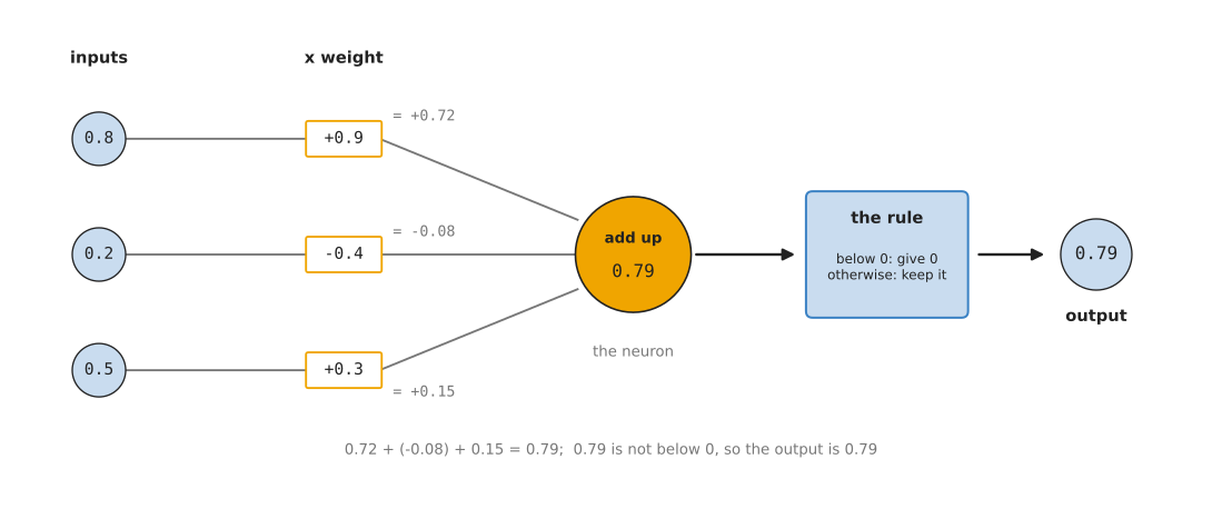
The inputs 0.8, 0.2 and 0.5 are multiplied by the weights +0.9, -0.4 and +0.3, the three results add up to 0.79, and because 0.79 is not below 0 the neuron's output is 0.79.
Here is the same calculation written out:
0.8 x 0.9    =  0.72
0.2 x (-0.4) = -0.08
0.5 x 0.3    =  0.15
                ----
total        =  0.79    ->  not below 0, so the output is 0.79
Now suppose the first weight were -0.9 instead of +0.9. The first line would be -0.72, and the total would be -0.72 - 0.08 + 0.15 = -0.65. That is below 0, so the neuron's output would be 0.
A real neuron usually also adds one extra number of its own to the total, before the rule, and this number is called the bias. The bias lets the neuron shift the point where it starts to give an output above 0, and it is learned in the same way as the weights.
This rule is called the activation function, and the neuron's output is called its activation. The rule described here, "below 0 becomes 0", is called the rectified linear unit (ReLU), and it is the most common one. But there are others with slightly different shapes, and they all do the same job.
The rule matters more than it looks, because without it every layer would only multiply and add. Many layers of multiplying and adding can always be replaced by a single layer that multiplies and adds, so extra layers would give the network no extra power. The rule breaks that, because once some outputs become 0 the network can behave differently for different inputs. That is what lets it learn complicated patterns, such as the difference between a mug and a bowl.
2. Layers, and why there are many of them#
Now that you know what one neuron does, a layer is simply a group of neurons that all read the same inputs. Each neuron in the layer has its own weights, so each one works out a different weighted sum, and the outputs of one layer are the inputs of the next.
The simplest network joins every neuron in one layer to every neuron in the next, and this is called a fully connected layer. The small network on the first page was made only of fully connected layers.
A network with many layers is called a deep network, and training one is called deep learning. There is no exact number of layers where "deep" starts, but networks for photos often have dozens of layers, and the largest language models have around a hundred.
Many layers help because each layer can build on what the one before it found. For example, in a network that reads photos, researchers have looked at what the neurons respond to. The early layers respond to simple things, such as an edge between dark and light, or a patch of one colour. Middle layers then respond to shapes built from those, such as a curve or a corner. Late layers then respond to whole parts of objects, such as a handle or a rim. Nobody tells the network to do this, because it comes out of training on its own.
3. How a picture becomes numbers#
A picture has to become numbers before any layer can touch it. The first page showed that a grey photo is a grid of brightness numbers, from 0 for black to 255 for white. This is why a colour photo has three such grids, one each for red, green and blue.
Before the numbers go into a network, they are usually scaled to be small. For example, they are divided by 255 so that they run from 0 to 1, because networks train better on small numbers. The photo is also usually resized to a fixed size, since a network expects the same number of inputs every time. Many networks for photos use 224 pixels by 224 pixels.
You could feed these numbers straight into fully connected layers, but that works badly for photos, for two reasons.
- It needs far too many weights, because a colour photo of 224 by 224 pixels is 150,528 numbers. So one fully connected layer of 1,000 neurons would need over 150 million weights, one for each input and neuron pair.
- It ignores where things are, because to a fully connected layer the pixel in the top left corner and the pixel next to it are no more related than any other two. So it would have to learn separately that a mug in the top left and a mug in the bottom right are both mugs.
So the next two sections describe the two kinds of layer that solve these problems.
4. Convolutional layers: small pattern detectors#
The first of those two kinds of layer solves both problems at once. A convolutional layer looks at a picture through a small window, often 3 pixels by 3 pixels, and the window has its own weights, one for each pixel in it. This small grid of weights is called a filter, and it works as a detector for one small pattern.
So the layer places the filter on the top left corner of the picture. It then multiplies each pixel under the window by the filter weight on top of it and adds the results, which gives one output number. Then it slides the window one pixel to the right and does the same again, and it repeats this at every position, row by row. The output is a new grid of numbers, a little smaller than the picture.
The picture below shows one filter sliding over a small picture that is dark on the left and bright on the right.
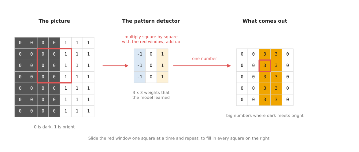
The filter gives 3 wherever its window covers the line between the dark part and the bright part of the picture, and 0 everywhere else.
Follow the red window, which covers three columns of the picture, 0, 0 and 1 in every row, while the filter's columns are -1, 0 and +1. So each row gives (-1 x 0) + (0 x 0) + (1 x 1) = 1, and the three rows together give 3, which goes in the matching square of the output grid.
Where the window covers only dark pixels, every product is 0, so the output is 0. Where it covers only bright pixels, each row gives -1 + 0 + 1 = 0. So the filter gives a big number only where dark changes to bright from left to right, which makes it a detector for that kind of edge.
In this example the filter weights were chosen by hand to make the idea clear, but in a real network the filter weights are learned by gradient descent, like every other weight. This means the network finds for itself which patterns are worth detecting.
A convolutional layer has many filters, often 64 or more, and each one detects a different pattern, so the output of the layer is one grid per filter. The next convolutional layer slides its own filters over those grids, so it detects patterns made of patterns. This is how the layers described in section 2 build up from edges to handles.
So convolutional layers solve both of the problems from section 3.
- They need few weights, because a 3 by 3 filter on a colour picture has 27 weights, and that same filter is used at every position in the picture.
- They treat every position the same way, so a filter that finds a handle in the top left finds it in the bottom right too, because it is the same filter.
This is why a network built mainly from convolutional layers is called a convolutional neural network (CNN). CNNs were the main kind of network for pictures from about 2012 until the early 2020s, and they are still widely used on robots because they are fast. ResNet, used in many robot models, is a CNN.
5. Transformers and attention#
A CNN is not the only kind of network used on pictures, so this section covers the other main kind. A transformer is a different kind of network from a CNN, and it was first built for sentences, in 2017, and is now also used for pictures, sounds and robot movements, so most of the large models in this book are transformers.
A transformer works on a list of pieces, and each piece is called a token.
- For a sentence, each token is a word or part of a word.
- For a picture, each token is a small square of the picture, called a patch, and a common choice is to cut the picture into patches of 16 pixels by 16 pixels. So a picture of 224 by 224 pixels becomes 14 by 14 = 196 patches.
- For robot movements, a token can be the arm's joint angles at one moment.
Each token starts as a list of numbers, and the key step in a transformer is called attention. In attention, every token looks at every other token and decides how much each one matters to it. Then it updates its own numbers by mixing in the numbers of the tokens that matter most.
The picture below shows attention for one word in a sentence given to a robot arm.
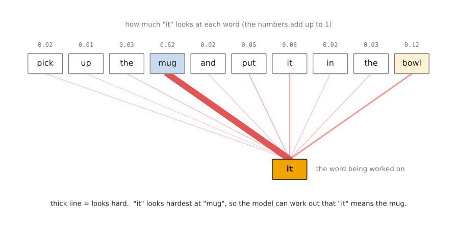
The word "it" looks at every word in the sentence; the thickness of each line shows how much, and the thickest line goes to "mug", which is what "it" means here.
The numbers above the words are how much "it" attends to each word, and they were made up for this picture to show the idea. In a real transformer they are worked out from the tokens, using weights learned in training, and they always add up to 1.
To understand the instruction, the robot needs to know what "it" refers to. The word "it" on its own does not say. So attention lets the token for "it" collect information from the token for "mug", and after this step the numbers for "it" carry some of the meaning of "mug".
Then a transformer repeats this many times, in many layers, and every token does it at the same time. Then each layer also has fully connected parts that work on each token separately.
For pictures, attention lets a patch showing the handle of a mug look at the patches showing the body of the mug, even when they are far apart. A convolutional layer only looks at a small window, so it needs many layers before distant parts of a picture can affect each other. Attention, however, links any two patches in a single layer. So a transformer that reads pictures as patches is called a vision transformer (ViT).
6. Embeddings: a list of numbers that stands for a thing#
Tokens carry lists of numbers through a transformer, and those lists have a name of their own. An embedding is a list of numbers that stands for a thing. That thing can be a word, a patch of a picture, a whole picture, a sound or a moment of robot movement.
So you have already met embeddings. The list of numbers that each token carries through a transformer is an embedding. So are the numbers that come out of the last layers of a CNN, just before the output, which form an embedding of the whole picture.
An embedding is usually a few hundred or a few thousand numbers long, and the numbers are not set by hand, because training finds them. A useful embedding has one important property: things that are alike get lists of numbers that are alike. So the embeddings for "mug" and "cup" are close together, while the embeddings for "mug" and "hammer" are far apart. Two photos of the same mug from slightly different angles also get close embeddings.
Here is a made-up example with only three numbers per embedding, to show what "close" means. The table lists four words and their made-up embeddings, so compare the rows to see which lists are alike.
| Thing | Made-up embedding |
|---|---|
| mug | 0.9, 0.8, 0.1 |
| cup | 0.8, 0.9, 0.1 |
| bowl | 0.7, 0.2, 0.2 |
| hammer | 0.1, 0.1, 0.9 |
The lists for "mug" and "cup" differ by only 0.1 in two places, so they are close. The list for "hammer" is different in every place, so it is far from all the others.
Embeddings are useful on a robot because distance can be measured. So if a model turns both pictures and sentences into embeddings of the same length, a robot can compare the sentence "a red mug" with every object it sees, and pick the object whose embedding is closest. The open-vocabulary models page describes models that do exactly this.
7. Encoders and decoders#
Embeddings are what one half of a model produces and the other half reads, so many models are built in two halves, and each half has a name of its own.
- The encoder reads the input and turns it into embeddings. For a photo, the encoder is often a CNN or a vision transformer, so its output is a set of embeddings that describe what is in the photo.
- The decoder reads those embeddings and turns them into the output the job needs: a label, a box, an outline, a sentence, or a list of arm movements.
Splitting a model this way is useful, because one encoder can then serve many decoders. An encoder trained on millions of photos learns embeddings that describe pictures well in general. You can then train a small decoder for your own job, such as finding where to grip a mug, on top of that encoder. This needs far fewer examples than training the whole network from nothing.
Some models are only an encoder, and some are only a decoder. For example, a model that turns a photo into one label can be an encoder with a tiny output layer. A language model that writes text one word at a time is a decoder, because it reads the words so far and gives the next word, again and again. You will see both words in the names of real models, such as the "image encoder" and "mask decoder" of the Segment Anything Model (SAM).
8. Layers that remember: sequence models#
Every layer so far looks at one input at a time, and a convolutional layer looks at one picture. But a robot often needs more than that, because it needs to know what happened a moment ago as well as what is happening now.
A sequence is a list of inputs in time order, such as the last 50 readings of a force sensor. So a sequence model is a network built to read a sequence and use the order of the readings. This section describes the three kinds that robot models use most: recurrent networks, convolutions along time, and state-space models. Transformers, from section 5, can also read sequences, so they are the fourth kind.
Why the past matters#
Think of a gripper holding a part, whose force sensor reads 3 newtons (N) now. Is the gripper squeezing harder, or is the part slipping out? The reading alone cannot say.
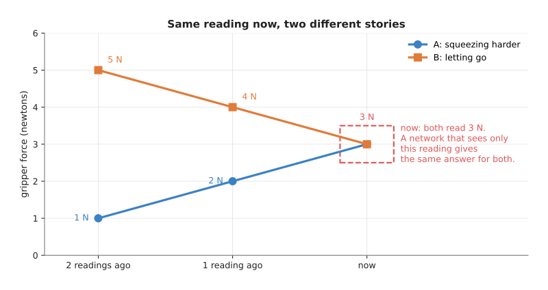
Story A rises to 3 N and story B falls to 3 N. A network that sees only the reading now gives the same answer for both.
The same is true for a movement policy, because one camera picture of an arm in mid-air does not show whether the arm is moving up or down. A force monitor, a program that watches the force readings for a collision or a slip, has the same problem. A single reading shows only how hard the grip is, while several readings show whether it is rising, falling or shaking. The force and slip models page shows what slip looks like in a force signal.
The simplest fix is to give a plain network the last few readings side by side, as one long input, and that works for a short, fixed window. But it breaks down when the window must be long, because the number of weights grows with every reading added. So the three kinds below handle long sequences better.
Recurrent networks: a memory passed from step to step#
A recurrent neural network (RNN) reads a sequence one step at a time. At every step it takes two inputs: the new reading, and a small list of numbers it kept from the step before. This list is called the hidden state, or simply the memory. The network uses the same weights at every step, and it gives out a new memory, which it passes on to the next step.
Here is a tiny recurrent rule, worked out in full. The memory starts at the first reading, and at every later step:
new memory = 0.6 x old memory + 0.4 x new reading
At the end, the network compares the reading now with its memory.
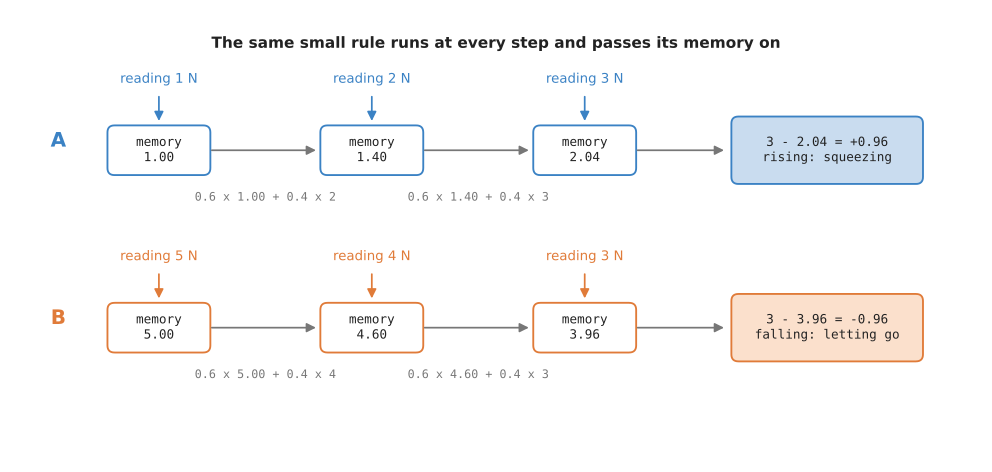
Both stories end on a reading of 3 N, but their memories differ, so the final answers differ.
A: readings 1, 2, 3   memory 1.00 -> 1.40 -> 2.04    3 - 2.04 = +0.96  rising
B: readings 5, 4, 3   memory 5.00 -> 4.60 -> 3.96    3 - 3.96 = -0.96  falling
In a real RNN the memory is a list of many numbers, the rule includes an activation function, and training finds the weights, while the 0.6 and 0.4 here were chosen by hand.
A plain RNN has a known weakness, because over a long sequence the effect of an early reading fades after many steps, and training struggles to reach it. The long short-term memory (LSTM) network, from 1997, fixes much of this by adding gates. Gates are small learned switches that decide at each step how much of the memory to keep, how much of the new reading to let in, and how much to pass to the output. The gated recurrent unit (GRU) is a simpler version with fewer gates, and both are still used in force and slip monitors, as the collision and failure detection page describes.
Convolutions along time#
Section 4 slid a small filter across a picture, and the same idea works along time. So a one-dimensional (1D) convolution slides a short filter along a list of readings.
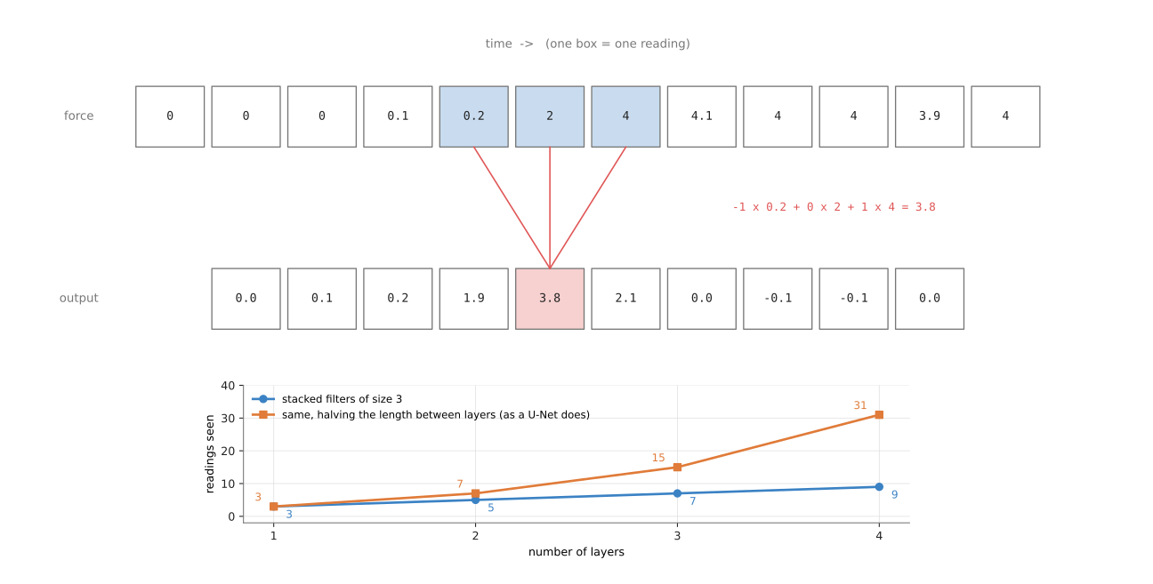
The filter -1, 0, +1 gives the change over two readings. It gives 3.8 where the force jumps from 0.2 N to 4 N, and about 0 where the force is steady.
The worked number for the highlighted position is:
-1 x 0.2 + 0 x 2 + 1 x 4 = 3.8
One filter of size 3 sees only 3 readings, so stacking layers is what widens the view. The small chart in the picture counts how many readings one output sees. With plain stacked filters of size 3, it is 3, 5, 7 and 9 readings after 1 to 4 layers. But if the list is halved in length between layers, it is 3, 7, 15 and 31.
Halving between layers is what a U-Net does. A U-Net shrinks its input step by step and then grows it back, and the segmentation page shows it for pictures. Diffusion Policy, a common movement model, uses a U-Net made of 1D convolutions along time. Its input is a short list of future arm positions, and the convolutions let each position take account of its neighbours, so the path comes out smooth. The diffusion and flow policies page explains that model.
Convolutions along time are fast, because every position is worked out at once rather than one step after another. Their cost is that they see only a fixed window.
State-space models: a running memory that can choose to forget#
Then a state-space model also keeps a memory and updates it at every step, like an RNN. The difference is that the update is a simple weighted sum with no activation function in between. That makes it much faster to train on long sequences, because the whole sequence can be worked out at once with a clever rearrangement of the sums.
So the simplest version of it is a running average:
memory = keep x old memory + (1 - keep) x new reading
With a fixed "keep" of 0.9, the memory changes slowly, which is good for smoothing noise and bad when something sudden happens. So Mamba, a state-space model from 2023, makes the model selective, which means the "keep" value is worked out from the new reading itself. The model can then learn to hold on to its memory while nothing is happening, and to throw it away when something important happens.
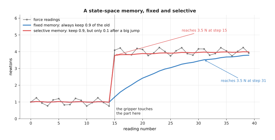
The gripper touches a part at step 15, and the fixed memory takes until step 31 to catch up. The selective memory, which keeps only 0.1 of the old value after a big jump, catches up at once.
In this picture the rule for "keep" was chosen by hand: 0.9, or 0.1 after a jump of more than 1 N. In Mamba, a small layer learns that rule from data.
Where they are used on a robot arm#
- A slip or collision monitor reads the last fraction of a second of force and current readings, so LSTMs and 1D convolutions are common here, because they are small and fast.
- Diffusion Policy's U-Net uses 1D convolutions along the time steps of the planned movement.
- Force and slip models shows a sequence model reading force and touch readings over time.
- Action chunking transformers use attention along time instead.
- Research policies such as MaIL and RoboMamba try Mamba layers in place of attention, to read long histories cheaply.
Where they fail#
An RNN or LSTM must work through the readings one after another, so training on long sequences is slow. A 1D convolution sees only its window, so an event older than the window is invisible to it. A selective state-space model is newer, and fewer ready-made robot models use it. Any sequence model also needs its readings evenly spaced in time. If readings arrive late or are dropped, the model sees a history that never happened.
Libraries#
PyTorch provides torch.nn.LSTM, torch.nn.GRU and torch.nn.Conv1d, which
cover the first two kinds. The mamba-ssm package from the Mamba authors
provides Mamba layers, but it needs an NVIDIA graphics card, because it uses
hand-written CUDA code. LeRobot includes a ready-made Diffusion Policy with
its 1D U-Net.
9. How big a model is: parameters#
All the numbers that training changes, the weights and the biases together, are called the model's parameters. So the number of parameters is the usual way to say how big a model is.
Counting them for a small network is simple, so take the network on the first page, fed with the 64 pixels of the 8 by 8 mug photo. It has 64 inputs, two hidden layers of 6 neurons, and 2 outputs.
weights:  64 x 6  +  6 x 6  +  6 x 2  =  384 + 36 + 12  =  432
biases:        6  +      6  +      2                    =   14
parameters:                                               446
Real models are far bigger, so the table below gives the size of four well-known models, from a photo network to a very large language model. Read the last column as the number of learned numbers stored in the model's file.
| Model | What it does | Parameters |
|---|---|---|
| ResNet-50 | a CNN that names the object in a photo | about 25 million |
| ViT-Base | a vision transformer that names the object in a photo | about 86 million |
| OpenVLA | reads a camera picture and an instruction, and outputs arm movements | about 7 billion |
| GPT-3 | a language model that writes text | about 175 billion |
A bigger model can learn more patterns, and usually needs more examples to train. It also takes more arithmetic every time it runs, so it is slower and needs a stronger computer. On a robot arm that must react many times a second, this matters a lot. The running-a-model page covers this choice.
10. Why these layers, and what they cost#
Now that you have seen all these kinds of layer, this section answers why networks use convolutional layers and transformers, rather than the obvious alternative of plain fully connected layers.
Fully connected layers are the simplest choice, and they are still used for short lists of numbers, such as the joint angles of an arm or the readings of a force sensor. But for pictures and sentences they fail, for the reasons in section 3: they need too many weights, and they cannot tell which inputs are next to each other.
A convolutional layer fixes both by sliding one small filter over the whole picture, but it costs you something too. Each filter sees only a small window, so the network needs many layers before it can connect distant parts of a picture.
A transformer fixes that with attention, which links every token to every other token in one step. Its cost is arithmetic, because every token looks at every other token, so doubling the number of tokens makes attention about four times as much work. Transformers also usually need more training examples than CNNs to reach the same accuracy on pictures, because they start with no built-in idea that nearby pixels belong together.
In practice, robot models use both. Small, fast models that must run many times a second on the robot often use CNNs, while large models that read pictures and instructions together are almost always transformers. Many models also join the two, with a CNN encoder for the camera pictures and a transformer on top.
For readings over time, the obvious alternative is again a plain fully connected layer, given the last few readings side by side, which is fine for a short window. The sequence layers in section 8 are for longer ones. An LSTM keeps a memory of any length, but it works one step at a time, so it is slow to train. A 1D convolution is fast, but it sees only a fixed window. A state-space model such as Mamba is fast and keeps a long memory, and its cost is that it is newer, with fewer ready-made robot models and a need for an NVIDIA graphics card.
11. Where to read next#
- Learning signals is the next page, and it explains the kinds of learning, from labelled examples to trial and error.
- Where the data comes from explains how the examples for robot models are collected.
- The map of models then shows the seven families of models in this book, and which of these layers each family uses.
- Image classification is the simplest seeing model: a CNN or vision transformer that names the object in a photo.
- Action chunking transformers shows a transformer whose tokens are camera pictures and arm movements.
- Foundation models in Book 3 describes today's very large models for robots, which are built from the layers on this page.
12. Using it in Python#
Section 1 worked one neuron out by hand, with the inputs 0.8, 0.2 and 0.5 and the weights +0.9, -0.4 and +0.3, and section 9 counted a model's parameters. This section builds the same kind of layer in PyTorch, so that you can see that the names in this chapter are the names of real classes. It shows the shape of the idea rather than a model worth training, because a network this small learns nothing useful.
import torch
from torch import nn

network = nn.Sequential(
    nn.Linear(3, 4),   # section 2's layer: 3 inputs into 4 neurons
    nn.ReLU(),         # section 1's rule: below 0 becomes 0
    nn.Linear(4, 2),
)

inputs = torch.tensor([[0.8, 0.2, 0.5]])              # one example, three numbers
print(network(inputs).shape)                          # torch.Size([1, 2])
print(sum(p.numel() for p in network.parameters()))   # 26

picture = torch.zeros(1, 3, 64, 64)   # one colour picture, 64 rows of 64 columns
conv = nn.Conv2d(in_channels=3, out_channels=16, kernel_size=3, padding=1)
print(conv(picture).shape)            # torch.Size([1, 16, 64, 64])
The number 26 is section 9's parameter count for this network, and you can check
it by hand. The first layer has 3 x 4 = 12 weights and 4 biases, and the second
has 4 x 2 = 8 weights and 2 biases, which comes to 26. The convolutional layer
turns 3 colour channels into 16 feature maps of the same height and width,
because padding=1 keeps the edges, and that is section 4's small pattern
detector as a single line.
The library gives you every layer type this page described, together with the
arithmetic and the random starting weights. Section 5's transformer block is
nn.TransformerEncoderLayer, its attention on its own is
nn.MultiheadAttention, section 6's embedding table is nn.Embedding, and
section 8's recurrent layer is nn.LSTM. You never write the multiplying and
adding yourself.
What you write is the arrangement: which layers, in what order, with what
widths. In practice almost nobody invents an arrangement, because a published
one that already works on a similar problem is a safer starting point, and
torchvision and Hugging Face's transformers package ship many of them ready
built.
What you have to decide is how many layers and how wide each one is, which activation to use, and which layer type suits your input. Section 2 explained why depth helps, and section 9 explained what depth and width cost, because the parameter count follows directly from those two numbers and it sets how much memory the model needs and how much data it takes to train.