The previous page ended with a problem: a policy that chooses one move at a time lets small mistakes add up until the arm drifts away from anything it was shown. This page explains ACT, which is short for Action Chunking with Transformers, and which was built to reduce that adding-up. ACT is a movement model that looks at the robot's cameras and chooses the next burst of moves all at once, instead of one move at a time. It was published in 2023 together with ALOHA, a cheap two-armed robot for recording demonstrations, and today it is the first policy most people train, usually through a software library called LeRobot.
The page answers five questions, in the order you would meet them. What does ACT take in, and what does it give out? How does the model work inside, once the data is in? How is it trained, and on how much recorded data? What are ALOHA and LeRobot, and why do they come up every time? And when is ACT the right choice for your own task?
It is for a reader who has read behaviour cloning, because ACT is a kind of behaviour cloning, and it was built to fix the problem of small mistakes adding up that is described there.
Contents#
- What ACT is
- What goes in and what comes out
- How it works inside
- How it is trained
- ALOHA and LeRobot
- Well-known models of this kind · 6.1 ACT in LeRobot, the one to start with · 6.2 The original ACT code, and one number it left behind · 6.3 The diffusion policy in LeRobot, when the routes disagree · 6.4 SmolVLA, a chunk from pretrained weights · 6.5 π0.5 in LeRobot, and what a slow chunk needs · 6.6 How to choose
- Where this is going
- Where to read next
1. What ACT is#
The introduction said that ACT chooses a burst of moves at once, and this section says what that burst is called and why it helps. In other words, ACT is a behaviour cloning policy that predicts a whole chunk of future moves at each decision.
A chunk is a short list of moves, one after another, and in ACT a chunk is usually 100 moves long. The arm makes 50 moves a second, so one chunk covers the next two seconds.
For example, when you pour water from a jug into a glass, you do not decide what to do every hundredth of a second. Instead you decide on the next second or so of pouring: tip the jug, hold it, start to tip it back. Then you look at the glass and decide again. So you make only a few decisions, and each one covers a stretch of movement.
So ACT does the same thing, and the picture below compares a policy that decides one move at a time with one that decides a chunk at a time.
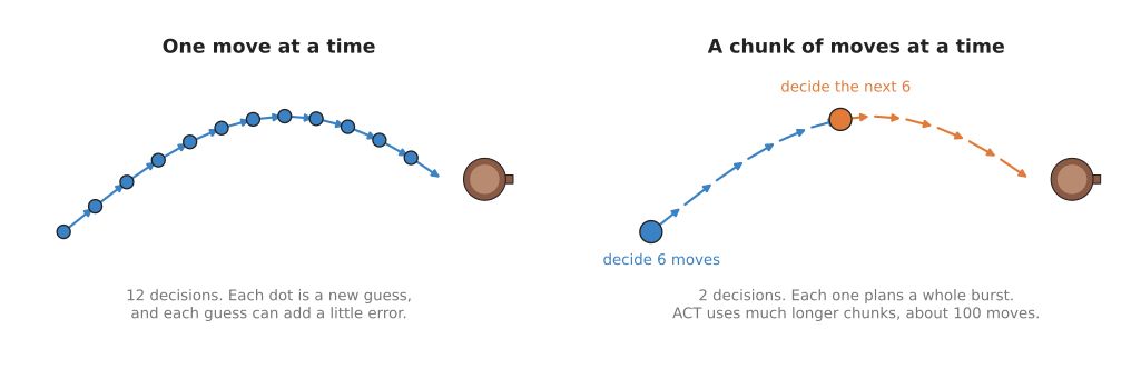
Each dot is one decision. But with one move per decision there are twelve chances for a small mistake, while with chunks there are only two.
This is why chunking helps with compounding error, which is the adding-up of small mistakes from behaviour cloning. Mistakes build on each other at each new decision, so fewer decisions means fewer chances for them to build up.
The other half of the name is transformer, which is a kind of neural network. It takes a set of pieces, such as parts of a picture, and it lets each piece take information from every other piece. The main step inside it is called attention, because for each piece the network works out which other pieces matter to it, and how much. Transformers were first used for text, and they are now used for pictures and actions too.
2. What goes in and what comes out#
Section 1 described chunks in general, and this section gives the exact numbers that the original ACT reads and writes. In the original ACT the robot is ALOHA, which has two arms, and each arm has six joints and a gripper. That makes 14 numbers in all, and together they describe where the robot is.
So the observation that ACT reads at each moment has two parts.
- Four camera pictures, each 480 pixels tall and 640 pixels wide, where one camera looks down from above, one looks from the front, and one sits on each wrist.
- The 14 current joint positions, which are six joint angles and one gripper opening for each arm.
The action is a chunk of 100 targets for each of the 14 joints, which is 1,400 numbers in all. Each target is a joint position the arm should reach at one moment in the next two seconds.
But the targets are joint positions rather than motor commands. So ordinary control code in each joint moves the motor towards each target, as described in the chapter overview.
3. How it works inside#
The three steps#
Section 2 said what goes in and what comes out, so this part follows the data between the two. When ACT runs on the robot, that data goes through three steps.
- An image encoder turns each picture into a grid of numbers. An encoder is the part of a network that turns its input into numbers the rest of the network can use. ACT uses ResNet-18, which is a small and well-known convolutional neural network (CNN). For each picture it gives a small grid, and each cell of that grid holds a list of numbers that describe one patch of the picture.
- A transformer compares every piece with every other piece. All the grid cells from all four cameras go into the transformer, together with the joint positions. Attention lets a piece from the wrist camera use a piece from the top camera, so this is how the network can match "the gripper is here" with "the cup is there".
- The transformer gives out the chunk. The last part of the transformer has 100 slots, one for each future moment, and each slot is turned into 14 joint targets.
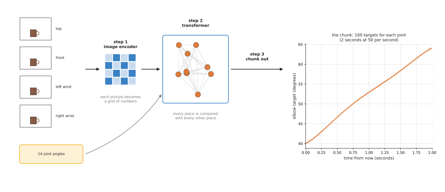
The plot on the right shows the chunk for one joint, the elbow, which is 100 targets, one every fiftieth of a second. The numbers in that plot are made up to show the shape, because a real chunk depends on the task.
These three steps are the policy that section 6.1 recommends, and the original code in section 6.2 holds the same network. The counts belong to the ALOHA rig of section 5: four cameras, 14 joint targets for two arms, and a chunk of 100. A cheap single arm has fewer of each, and the other models in section 6 keep the three steps and change the numbers. SmolVLA, in section 6.4, and π0.5, in section 6.5, also add one input that the steps above do not have, which is a sentence saying which task to do, and they read it in the same transformer that reads the pictures.
The style numbers#
The three steps above give one chunk for one situation, but people do the same task in slightly different ways. For example, one time the demonstrator moves quickly, and another time slowly. As the behaviour cloning page shows, a network that has to give one answer blends these ways together.
But ACT has a partial fix for this problem. During training only, a second small network looks at the real chunk the person made, and it sums up "how the person did it this time" in a few numbers. On this page we can call those few numbers the style numbers. The main network gets the style numbers as an extra input. So it does not have to blend different styles, because the style numbers tell it which one to produce.
At run time there is no person, so there is no real chunk to look at. ACT therefore sets the style numbers to zero, which stands for the most typical style, and the result is a smooth, typical movement.
This design has a name, which is a conditional variational autoencoder (CVAE). However, you do not need the details of it to use ACT. The idea is only that some of the variation between demonstrations is put into separate numbers, so that it does not blur the actions.
It is only a partial fix, because setting the style to "typical" at run time still gives one answer. So if half the demonstrations go left of an obstacle and half go right, ACT can still struggle. But the diffusion and flow policies on the next page handle that case better, and the one to reach for is the diffusion policy in section 6.3, which sits in the same library and takes the same recordings.
Blending overlapping chunks#
A chunk covers two seconds, so if the arm plays the whole chunk without looking again, it cannot react to anything that happens during those two seconds. There are two common ways to run ACT, and they differ in how they handle that.
The first way is to play part or all of a chunk, and then ask the policy for a new one. This is simple, but the arm can jump a little where one chunk ends and the next begins.
The second way is to ask the policy for a new chunk at every step, and then blend the chunks together. The ACT paper calls this temporal ensembling, because "temporal" means to do with time, and "ensembling" means combining several guesses into one.
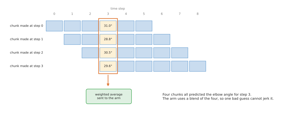
At step 3, the chunks made at steps 0, 1, 2 and 3 all hold a target for step 3, so the arm uses a weighted average of them. A weighted average is an average where some values count for more than others. This makes the movement smooth, because one odd guess is outweighed by the others.
4. How it is trained#
Section 3 described the network, and this section describes how its numbers are fixed. ACT is trained like any behaviour cloning policy, with one change: the answer is a whole chunk, and not one move.
The data is a set of demonstrations, as it is for plain behaviour cloning. At each moment of each demonstration, the training program takes the pictures and joint positions as the question. Then it takes the next 100 recorded joint positions as the answer. The loss is the size of the difference between the predicted chunk and the recorded chunk, added up over all 1,400 numbers. The training program then nudges the network to make that loss smaller.
So how much recorded data does this training actually need? In the ACT paper, each task was learned from about 50 demonstrations, which is about ten minutes of recording. The tasks were fine two-handed tasks, such as opening a small plastic cup with a lid and slotting a battery into a holder. This is much less data than people expected fine tasks to need, and that is the main reason ACT became popular. The Book 3 page on data and demonstration gives the reported success rates, and it warns what they do and do not show.
Training runs on one ordinary graphics card, so it does not need a cluster of computers.
5. ALOHA and LeRobot#
Sections 2 and 4 both mentioned ALOHA and LeRobot, so this section says what they are. ACT is closely tied to these two names, and you will meet both whenever you read about it.
ALOHA is the robot ACT was built for, and the name is short for A Low-cost Open-source Hardware System for Bimanual Teleoperation, where "bimanual" means using two hands. ALOHA has two follower arms, which do the task, and two smaller leader arms, which a person holds and moves by hand. Each follower joint copies the matching leader joint, and there are four cameras.
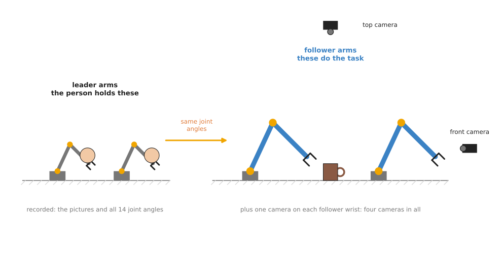
The person moves the grey leader arms. Then the blue follower arms move to the same joint angles and do the task, while the cameras and joint sensors record everything.
This way of recording has one large advantage over a joystick. The person's hands do the task directly, joint for joint, so they can control all 14 joints at once. This is very hard to do in any other way. The follower arms in the original ALOHA are ViperX arms and the leader arms are WidowX arms, both sold by Trossen Robotics. The designs were published openly, so other groups could build the same robot.
LeRobot is a free software library from the company Hugging Face, first released in 2024. It holds, in one place, a standard way to store robot recordings, the code to train several kinds of policy, and drivers for cheap robot arms. ACT is one of its policies, and LeRobot's own documentation calls ACT its recommended first policy. The Book 3 page on LeRobot explains why it became the standard place to start.
LeRobot also works with cheap leader-and-follower arms, such as the SO-101. These use the same leader-and-follower idea as ALOHA, but with small hobby motors and 3D-printed parts. A pair costs a few hundred dollars, so a person can record ACT demonstrations at home.
6. Well-known models of this kind#
Section 5 described the ALOHA rig and LeRobot. This section names the chunk-predicting policies you can actually obtain, says which one to reach for first, and gives for each one the shortest command or program that does something real with it.
The hardware in this line is not in the table, because the table is about models. ALOHA itself is in section 5. Mobile ALOHA (2024) put the same arms on a wheeled base and trained ACT on tasks that need the robot to move around a room, and ALOHA 2 (2024), from Google DeepMind, is a sturdier redesign whose designs and simulation model were published.
Read the table as a filter rather than as a ranking. The left column names the model
and says how much use it gets. The right column holds what you filter on: what it is
best at, its size, its licence, whether it trains on an Apple Silicon Mac with no
separate graphics card, and when to pick it. Find the row that matches the hardware
you have, then read that model's sub-section. A size is the number of trainable
values that the project itself states, and it says not stated where no project
document gives a figure. The answers about the Mac come from LeRobot's
compute hardware guide, which
groups policies by the video memory they need to train at a batch size of eight.
| Model | What decides it |
|---|---|
| ACT in LeRobot (2023), most used in 2026 | It is best at one careful task on your own arm, trained from nothing. It has about 80 million trainable values, and it is Apache-2.0. It trains on a Mac in about 6 to 14 hours. Pick it when you have an arm, two cameras and about 50 recordings. |
| The original ACT code (2023), historical | It is best at reading the implementation the paper was written from. It has about 80 million trainable values, and it is MIT. Whether it trains on a Mac is not stated. Never pick it for a project, and open it only to read. |
| Diffusion policy in LeRobot (2023), most used in 2026 | It is best at tasks where the demonstrations disagree about the route. Its size is not stated, and its licence is Apache-2.0 in LeRobot and MIT for the original. Training it on a Mac is marginal, because it needs about 8 to 14 GB. Pick it when your ACT policy wavers between two routes. |
| SmolVLA (2025), worth betting on | It is best at starting from trained weights, and at being told the task in a sentence. It has 450 million trainable values, and both its code and its weights are Apache-2.0. Running it on a Mac works, and training it there is marginal. Pick it when fifty recordings are not enough, or when one policy must do several tasks. |
| π0.5 in LeRobot (2025), worth betting on | It is best at working in a room it was not trained in. Its size is not stated, its code is Apache-2.0, and the weights LeRobot serves carry Gemma terms. It does not train on a Mac. Pick it when you can rent a large card and need that generalisation. |
6.1 ACT in LeRobot, the one to start with#
Most used in 2026. Size s, a small card, Apache-2.0, and no weights to download, because the ACT policy you run is always one you trained yourself.
This is the version of ACT that nearly everybody runs. LeRobot implements the network from the paper Learning Fine-Grained Bimanual Manipulation with Low-Cost Hardware, and its page for the policy calls it "the first model we recommend when you're starting out", and says it often reaches a high success rate with 50 demonstrations. It is in the base LeRobot installation, so there is no extra dependency to install for it.
The one idea that separates ACT from every other row of the table is that it produces its chunk in a single pass of a single network. The three steps of section 3 run once, and the hundred commands are there. The original ACT code in section 6.2 is the same network, but every other policy in the table builds its chunk the other way, by starting from a chunk of random numbers and improving it over several passes. The sub-sections below describe each of those in turn, and almost everything else in the table follows from this one difference.
What that changes inside is the training target and what comes back at run time. Training compares the predicted chunk with the recorded one and adds up the plain distance between the two, number by number, without squaring it. That choice matters in a way that is easy to see with one number instead of fourteen hundred. If you have to pick a single number to stand for many, the one with the smallest total distance to all of them is the middle number of the list, while the one with the smallest total squared distance is their average. ACT is trained on plain distance, so the chunk it settles on leans towards the middle of the chunks it was shown rather than their average, and one unusual demonstration drags it less far. It is still a single chunk, though. The style numbers of section 3 are set to zero when the policy runs, so the chunk is decided entirely by the pictures and the joint positions: the same observation gives the same chunk, every time.
What the single pass buys is cost and repeatability. ACT is the cheapest row of the table to train and the quickest to answer, which is why it is the only one you can train overnight on a laptop, and why it never needs the real-time chunking that section 6.5 has to describe for the large policies. Because its answer is decided by the observation alone, a failure repeats: you can run the same attempt again, see the arm do the same wrong thing, change one setting and compare. You cannot do that with the diffusion policy of section 6.3 or with SmolVLA in section 6.4, where the chunk starts from fresh random numbers and two attempts from the same picture differ. What the single pass costs is that one chunk is one answer, and the style numbers do nothing about that at run time, because they are asked for the typical way of doing the task.
On a robot arm the choice shows up as soon as you look at who recorded your demonstrations. Fifty recordings of one careful motion, made by one person who did it the same way each time, are what ACT was built for, and the diffusion policy would cost you a bigger card and a longer training run for a result you could not tell apart. Two people who approached the object from different sides, or one person who changed their mind halfway through the session, give you recordings that disagree, and ACT's one chunk then lands between the two approaches. Section 6.3 is the row for that case.
You would pick ACT over the diffusion policy in section 6.3, which is the obvious alternative and the other chunk-predicting policy in the same library, because it is the cheaper of the two by a clear margin, as the size and machine lines of the two sub-sections show. Both choose a chunk, so you lose nothing about the subject of this page by starting with the cheaper one.
What it costs you is a recording session and the pair of numbers below. There is no pretrained ACT policy that transfers to you, because the output layer has one number per joint of the arm it was trained on, so a policy trained on a seven-joint Franka arm cannot even be loaded for a six-joint SO-101.
Training is a command rather than a program, because LeRobot reads the number of joints and the number of cameras from your recording and sizes the network to fit.
# chunk_size is how many future commands the network predicts in one pass, and
# n_action_steps is how many of them the arm carries out before asking again.
lerobot-train \
  --policy.type=act \
  --dataset.repo_id=${HF_USER}/my_dataset \
  --policy.chunk_size=100 \
  --policy.n_action_steps=50 \
  --output_dir=outputs/train/my_act \
  --job_name=my_act \
  --policy.device=cuda
The program below then runs what that produced, and it is the smallest piece of code that shows the chunking this page is about.
from lerobot.datasets import LeRobotDatasetMetadata
from lerobot.policies import make_pre_post_processors
from lerobot.policies.act import ACTPolicy

checkpoint = "outputs/train/my_act/checkpoints/last/pretrained_model"
policy = ACTPolicy.from_pretrained(checkpoint)
print(policy.config.chunk_size, policy.config.n_action_steps)

# The rescaling of inputs and outputs is built from the recording's own statistics.
meta = LeRobotDatasetMetadata("<my-user>/my_dataset")
preprocess, postprocess = make_pre_post_processors(policy.config,
                                                   dataset_stats=meta.stats)

policy.reset()      # empties the queue of unused commands from the last attempt
batch = preprocess(frame)   # frame is one observation, as tensors on the device

# The whole chunk at once, which is what the network really produces.
chunk = policy.predict_action_chunk(batch)

# Or one command at a time, taken from a queue that is refilled when it empties.
action = postprocess(policy.select_action(batch))
chunk_size is how many future commands the network produces in one pass, and its
default in LeRobot is 100. n_action_steps is how many of those the arm carries out
before the policy is asked again, it defaults to 100 as well, and it must not be
larger than chunk_size. select_action hides the difference between the two: it
keeps a queue, returns the next command from it, and runs the network again only when
the queue is empty, so calling it once per control step gives you the chunking without
writing the bookkeeping. policy.reset() empties that queue between attempts, and
predict_action_chunk is there when you want the whole chunk yourself. frame is
your robot's cameras and joint readings turned into tensors, which LeRobot's
build_inference_frame helper does from a raw observation and the recording's field
list.
What LeRobot gives you is the network from the paper, the training loop, the queue,
the rescaling, the checkpoints and the control loop on the arm. What you supply is the
recordings, and ACT is the model where that is least avoidable, because it was
designed for tasks that need care and those are the tasks where a demonstration has
to be good. You also supply the pair of numbers above, and section 3 explains the
trade between them. If you want the blending of overlapping chunks that section 3
described, temporal_ensemble_coeff turns it on, and LeRobot then requires
n_action_steps to be 1, because blending means running the network at every single
step.
6.2 The original ACT code, and one number it left behind#
Historical. Size s, a small card, MIT.
The code the paper was written from is still online, and reading it is the only reason to open it. Checked on 3 October 2026, its last change was in July 2024 and it has not been archived, so it is dormant rather than withdrawn.
The network inside it is the network of section 3, so this sub-section is the one place on the page where the answer to "how is this one different inside" is "it is not". The one idea here is that research code is written to produce one paper's results on one rig, and everything about it follows from that. The recording format is the authors' own, the robot side talks to the ALOHA arms of section 5 through ROS and a second repository, and the versions are the versions that worked in 2023.
There is, though, one real difference inside, and it is worth knowing because it is
about the chunk. The transformer that produces the chunk has a second half, called the
decoder, which is the part holding one slot per future moment. Stacking several decoder
layers lets those slots be revised several times before they are read out. LeRobot's ACT
configuration sets n_decoder_layers to 1, and its own comment explains why: the
original implementation asks for 7, but a bug in that code means only the first of the
seven is ever used, so LeRobot sets 1 to match what the original actually did. The
comment links to the issue in the original repository where this was found. Everything
else in LeRobot's defaults is the paper's: a ResNet-18 picture encoder, a model width of
512, four encoder layers and a chunk of 100.
What the difference buys you is nothing, and what it costs is the risk of a comparison that means nothing. If you read the paper, built its 7-layer decoder yourself, and measured it against LeRobot's single layer, you would be comparing two different networks and attributing the gap to the library. The general lesson is worth more than the setting, and it is the reason this row is in the table at all. When a paper's number and a maintained library's number disagree, the library has usually read the paper's code, and the code is what produced the result.
You would not pick this repository over LeRobot's version, and the reason is not the
network. It is everything around the network. LeRobot gives you one recording format,
drivers for cheap arms, a training script that sizes the network from your recording,
and a control loop that runs the result at a fixed rate. The original code supplies
none of that. Its own installation instructions pin Python 3.8.10, MuJoCo 2.3.7 and
dm_control 1.0.14, and they install rospkg, because its real-robot side runs through
ROS. What it costs you, if you use it anyway, is all of the work LeRobot does for you,
on top of a set of pinned versions from 2023 that an environment built today has to be
made to accept.
# The paper's settings written out, although these are LeRobot's defaults already.
# Note n_decoder_layers: 1, not the 7 the original code appears to use.
lerobot-train \
  --policy.type=act \
  --dataset.repo_id=${HF_USER}/my_dataset \
  --policy.vision_backbone=resnet18 \
  --policy.dim_model=512 \
  --policy.n_encoder_layers=4 \
  --policy.n_decoder_layers=1 \
  --policy.chunk_size=100
Whichever one you run, the chunk is the same chunk, which is why this row changes nothing about the subject of the page.
6.3 The diffusion policy in LeRobot, when the routes disagree#
Most used in 2026, alongside ACT, and it is the other policy a beginner is likely to train. Size not stated, a big card, Apache-2.0 in LeRobot and MIT for the original Stanford code.
A diffusion policy also predicts a chunk, so everything on this page about chunk length still applies to it. What it changes is how the chunk is produced. The next page is about that in full, and the four paragraphs here say only how it differs from ACT.
The one idea is to stop asking the network for the right chunk and ask it instead to improve a wrong one. The network then has a much easier question to answer, which is "this chunk is slightly wrong, in which direction", and a network that answers that question can be run again on its own answer. Run it enough times, starting from a chunk of random numbers, and what you end up holding is one of the chunks the recordings contained, rather than something between them.
Inside, this is a different machine from ACT's and not a changed setting. ACT turns each camera picture into many pieces and lets each future moment of the chunk look at each piece. LeRobot's diffusion policy instead flattens everything it knows about the situation, which is the picture features from the two most recent observations together with the joint positions, into one long list of numbers. That list then steers a convolutional network which runs along the time axis of the chunk, squeezing its moments down into fewer and longer ones, mixing them, and expanding them back out. Which round of the cleanup it is doing is also an input, so one network serves every round. Training adds a random amount of noise to a recorded chunk and asks the network to name the noise that was added. Running starts from pure noise and takes off what the network names, round after round. The whole network therefore runs once per round, where ACT's runs once per chunk, and that is where the memory and the time in the line above go.
What the design buys is that the policy describes a spread of good chunks instead of one chunk. If some of your recordings go left round an obstacle and others go right, each round of the cleanup pulls the chunk towards whichever of the two it is already nearer, so a run comes out as a whole left chunk or a whole right chunk and never as half of each. ACT cannot do that at run time. Its style numbers hold the variation between demonstrations aside while it trains and are then set to the typical value, so the one chunk it gives back sits between the two routes, which on a table with an obstacle means through the obstacle. What the design costs, besides the training, is the repeatability that section 6.1 counted as ACT's advantage: the noise is drawn fresh for every chunk, so the same picture gives a different motion each time, and a failure you want to investigate may not happen again.
On a robot arm the difference decides the result when more than one person recorded your demonstrations, or when one person changed their approach during the session. Train ACT on those recordings and the arm drives into the obstacle both people went around. Train the diffusion policy on the same file and it picks a side. The difference costs you when the opposite is true: fifty recordings of one route by one person give the diffusion policy nothing to choose between, and you have paid a bigger card and a longer training run for a spread with one thing in it.
You would therefore pick it over ACT when your demonstrations disagree about the route, and ACT over it when they do not.
What it costs you is one extra install, because the policy depends on the diffusers library.
pip install 'lerobot[diffusion]'

lerobot-train \
  --policy.type=diffusion \
  --dataset.repo_id=${HF_USER}/my_dataset \
  --output_dir=outputs/train/my_diffusion \
  --job_name=my_diffusion \
  --policy.device=cuda
Everything else is the same as ACT, which is the point of a library with one training script. Once the extra package is installed the command differs by one word, so training both on the same recording and comparing them takes an afternoon rather than a project.
6.4 SmolVLA, a chunk from pretrained weights#
Worth betting on, because starting from trained weights is where the field has gone, and this is the one example of it that a small machine can run. Size m, a laptop to run it and a big card to train it, Apache-2.0 for the code and for the weights.
SmolVLA was released by Hugging Face in June 2025. Book 3's page on foundation models records that it pairs a vision-language backbone with a smaller action-producing part and reports about 78 per cent success on real SO-100 arm tasks. It predicts a chunk, and its configuration in LeRobot sets that chunk to 50 commands rather than ACT's 100.
The one idea is that the hard part of reading a scene has already been paid for by somebody else. ACT's picture part is a ResNet that was trained to name the objects in ordinary photographs, and it knows nothing about words. SmolVLA keeps a whole vision-language model instead, which is a network trained on pictures paired with text, and attaches a smaller network called the action expert to produce the moves. So the pictures, the sentence naming the task, and the arm's own joint positions all enter the same stream of pieces for the big network to read, where each picture is compressed to a small number of pieces and the joint positions are turned into a single piece by one layer.
The action expert is about three quarters as wide as the big network, and inside it the layers alternate between looking at what the big network produced and looking at the other moves of the chunk being built. Two choices in its announcement are what make a model of this size run on a small machine at all. The expert reads the big network only up to the middle of its layers, rather than waiting for its last one, which halves the work of both parts. And at run time only the whole picture is used, rather than the several cropped tiles the vision-language model was pretrained with.
The chunk itself is produced by a third method, which is neither ACT's single pass nor the rounds of cleanup in section 6.3. It is called flow matching. During training, noise is mixed into the recorded chunk, and the expert is asked for the correction that points from the noisy chunk straight back to the recorded one. Because that correction points straight at the finished chunk rather than along a winding path, following it at run time takes only a few steps, and LeRobot's configuration uses ten of them, where the diffusion policy's default cleanup runs many times more. The pictures and the sentence go through the big network once and the result is held, so only the small expert repeats, which is why ten steps are affordable here and a hundred would not be. Like the diffusion policy and unlike ACT, the chunk starts from fresh random numbers, so SmolVLA can give one of several good chunks instead of the middle of them.
This buys the two things ACT cannot do. Its weights already exist, so your recordings adjust a policy that has seen many people's robots instead of creating one from nothing. And it reads a sentence, so one policy can be told at run time which of several jobs you want, where an ACT policy trained on several tasks has no input to tell it. What it costs is that the big network has to be loaded and run even though only the expert produces the moves, which is the whole of the difference in the machine line above. On a robot arm the difference shows up when one arm has to do two jobs. With ACT you would train one policy for each and choose between them in your own code, and with SmolVLA you train once and change the sentence you pass in.
What it costs you besides that is an extra install and attention to the task text. That text must match the words used when recording, because it is an input to the network rather than a label for you.
pip install 'lerobot[smolvla]'

# Fine-tune the pretrained policy on your own recording.
lerobot-train \
  --policy.path=lerobot/smolvla_base \
  --dataset.repo_id=${HF_USER}/my_dataset \
  --batch_size=64 \
  --steps=20000 \
  --output_dir=outputs/train/my_smolvla \
  --job_name=my_smolvla \
  --policy.device=cuda

# Run it, and give the task in the same words the recording used.
lerobot-rollout \
  --strategy.type=base \
  --policy.path=outputs/train/my_smolvla/checkpoints/last/pretrained_model \
  --robot.type=so101_follower \
  --robot.port=/dev/ttyACM0 \
  --task="Put the cup in the box" \
  --duration=60
What Hugging Face gives you is a policy that has already seen 487 people's robots, so your recordings only have to teach it your room. What you supply is still the recordings, the sentence, and a card to train on.
6.5 π0.5 in LeRobot, and what a slow chunk needs#
Worth betting on, as the direction rather than as this weekend's work. Size not stated, a workstation, Apache-2.0 for the openpi code and the Gemma terms of use for the weights LeRobot serves at lerobot/pi05_base, read on 3 October 2026.
π0.5 is a vision-language-action policy from Physical Intelligence. LeRobot's page for it describes its aim as working in places it was never trained in, and says the LeRobot version is adapted from the company's open openpi repository. Like everything else on this page it produces a chunk, and LeRobot's own quickstart for it carries 10 commands out of each chunk.
The one idea is that generalisation comes from the training mixture rather than from the network. The chunk is produced much as SmolVLA's is, by a vision-language model with a flow-matching action expert attached, so this row is not here for its architecture. It is here for what it was trained on. Its paper describes co-training on tasks of different kinds at once: pictures from the web with captions, questions and answers about those pictures, where objects are in them, people telling a robot the next step in words, the names of the subtasks a long job breaks into, recordings from several different robots, and recordings from many different homes.
What that changes inside is what counts as an answer. ACT has one kind of output, which is a chunk of joint targets, so every training example must be a chunk. π0.5 is trained on examples whose answer is sometimes a chunk and sometimes a piece of text, such as the name of the next subtask, and the same network produces both. The arm's own posture enters the same way. LeRobot's page says the joint positions are put on a scale of 256 whole numbers and written into the prompt as text, where ACT feeds them in as numbers and SmolVLA turns them into one piece by a single layer. So to π0.5 the robot's state, the task and the next subtask are all words in one stream, and that is what lets web pictures and robot recordings train one network.
What this buys is the one thing no other row of the table promises, which is working in a place it was never trained in, because a model that has read captions of kitchens it never worked in has somewhere to start when it sees a new one. What it costs is a rented card rather than anything on your desk, and one thing that stops the first training run before it begins: the backbone's tokenizer is a gated model on the Hugging Face Hub, so you must accept its licence and sign in before training will begin. On a robot arm the difference shows up in exactly one situation. Your ACT policy works on your table, and then somebody moves the table or opens the blind, and it stops working. ACT has no answer to that other than recordings of more rooms, which is what a policy pretrained on many rooms already has.
pip install 'lerobot[pi]'
hf auth login          # the backbone's tokenizer is gated; accept its licence first

lerobot-train \
  --policy.type=pi05 \
  --policy.pretrained_path=lerobot/pi05_base \
  --dataset.repo_id=${HF_USER}/my_dataset \
  --policy.n_action_steps=10 \
  --policy.gradient_checkpointing=true \
  --policy.dtype=bfloat16 \
  --policy.device=cuda
One more thing here belongs to this page rather than to π0.5. A large policy takes
longer to produce a chunk than the arm takes to carry the chunk out, so there is a
pause or a jerk every time a chunk arrives late. LeRobot's answer is called real-time
chunking, described on its own page: the
next chunk is produced while the arm is still carrying out the current one, and the
beginning of the new chunk is pulled towards the part of the old one already played,
so the two join smoothly. It is turned on with --inference.type=rtc, it works for
π0, π0.5 and SmolVLA, and it is the reason chunking still works with a model that
takes a long time to produce each chunk.
6.6 How to choose#
The default is ACT in LeRobot. Record about 50 demonstrations of one task on a cheap leader-and-follower arm, train ACT with its default chunk of 100 and half of that carried out, run it on the arm, and watch where it fails.
Three failures change the choice, and each points at a different row. If the arm wavers between two routes, or stalls where your recordings disagreed, train the diffusion policy instead, and read the next page before you do. If fifty recordings are not enough, or if one policy has to be told which of several tasks to do, fine-tune SmolVLA. If the policy works in your room and fails in the next one, you need a policy pretrained on many rooms, and that means π0.5 and a rented card rather than anything you can train this weekend.
Two limits sit under all of that. On an Apple Silicon Mac, ACT is the only row of the table that finishes in a night, so start there whatever your task looks like. And the original ACT code is never the answer: whatever you choose, run LeRobot's version.
The idea of predicting a chunk spread well beyond ACT itself. Every policy in the table above produces one, and so do the large vision-language-action models. The question is no longer whether to chunk, but how long the chunk should be and how to join one to the next.
7. Where this is going#
This section is about where chunk-predicting policies are heading. It is written on 4 October 2026, and it uses the vocabulary that Book 3's frontier chapter sets out for the four kinds of claim. A demonstration is a recording of something working once under conditions the publisher chose. A product announcement says a thing can be bought or downloaded, and you can check it, which makes it the most useful kind. A research result is a measured number under a stated protocol. A projection is a statement about a date that has not arrived, and it is the weakest. Each claim below says which kind it is, and where the judgement is mine the sentence says so.
How it got here#
ACT arrived in 2023 as one paper's answer to one problem, and what happened next was not that ACT improved. ACT barely changed. Instead its output shape spread: predicting a burst of future commands in one pass, rather than one command at a time, became something almost every new policy does, including policies that share nothing else with ACT. Section 6.6 put it as the question no longer being whether to chunk. The work since has gone into what else the chunk should contain and how to join one chunk to the next.
Where it is used in industry today#
ACT itself is not a product and nobody sells it. Its industrial presence is indirect, and there are three honest ways to see it.
The first is the hardware. The rig that the ACT paper introduced became a product line: Trossen Robotics sells its descendants as the Stationary AI two-arm kit at $23,995.95 and the Mobile AI version at $33,695.95. Read those pages carefully, because Trossen retired the ALOHA brand in March 2025 and the legacy line reached end of life on 1 July 2025, while the current products still carry "Aloha" inside their full names.
The second is the library. LeRobot is Apache-2.0 and ships ACT as one policy among about ten, with one dataset format and one training command, and it is what NVIDIA chose when it put GR00T N1.7 and a teleoperation framework into it on 6 July 2026. That is a vendor with its own stack deciding that somebody else's library is where its model should live, which tells you more about adoption than any download figure.
The third is the chunk inside commercial policies. Google DeepMind's Gemini Robotics 2 offers its reasoning model through Google AI Studio and keeps the two models that actually move a robot with early-access partners. Figure's Helix 2.5 reports 56 per cent zero-shot success across 30 unseen homes against 9 per cent for the same architecture trained from scratch, and nothing about it is downloadable, so it is a research result and not a product. Skild AI's S1 is in commercial use with partners and cannot be obtained. The pattern is the one Book 3 records in its section on what none of them can do: the frontier chunk predictors are demonstrated and closed, and the open shelf trails them by roughly eighteen months.
What is being worked on right now#
Four fronts are active, and three of them are attempts to put something into the chunk that ACT's chunk does not contain.
The largest is force. ACT predicts positions, and a position says nothing about how hard to push, which is why Gemini Robotics 2's own numbers show 92 per cent at unscrewing a light bulb and 36 per cent at screwing one in. Taking apart needs position control and putting together needs force control. CompVLA predicts a stiffness matrix alongside the motion, so the model that decides where to go also decides how hard to push, and ForceRFT refines a policy's actions using force-guided reinforcement learning. Both are September 2026 papers with measured results and no released product. This is the front I would watch most closely, because it is the one with a named commercial reason behind it.
The second is memory. A chunk is chosen from the current observation, so two moments that look the same produce the same chunk even when the task needs different actions. Book 3 records several September 2026 submissions adding persistent state to policies for exactly this reason, in its section on current research directions. It is the least glamorous of the four and probably the most consequential for long tasks, because a policy that cannot remember what it already did cannot recover from its own mistakes.
The third is making the chunk predictor small enough to run on the robot. FoldQuantVLA reports four-bit weights and four-bit activations with speedups of 1.20 to 1.33 times. Quantisation means storing each number with fewer bits so the model fits in less memory. This front has an external cause with a date attached: NVIDIA announced three Jetson Thor computers on 15 July 2026 with physical hardware stated for the first quarter of 2027, the entry-level part has 16 gigabytes of memory, and current large policies do not comfortably fit in it. That is a product announcement creating a research problem.
The fourth is where the chunk predictor's weights come from. ACT is trained from nothing and the newer chunk policies are not. SmolVLA puts a roughly 100-million-parameter flow-matching action expert on a vision-language backbone and reports about 78 per cent success on real SO-100 arm tasks. MolmoAct2, from the Allen Institute for AI, grafts the same kind of expert onto an autoregressive vision-language model, and GigaBrain-0.7 is Apache-2.0 on both code and weights. All three are downloadable, which puts them in a different class from the closed models above.
What is still unsolved#
Nobody has shown a reliable way to tell whether a chunk policy will work before running it on the arm, and this is the problem that has resisted the most effort. The research result that makes it concrete is LIBERO-VPro, a September 2026 study of six foundation models across 12 categories of visual disturbance, roughly 196,000 simulated episodes and 200 real trials on a Franka Research 3 arm. It found that the models tolerated whole objects being hidden, degraded sharply when the small local cues at the point of contact were disturbed, and were very sensitive to stale or missing camera frames. A chunk makes this worse, because the policy commits to a burst of commands and carries them out without looking, so a disturbance arriving mid-chunk is acted on only when the next chunk is chosen. An August 2026 survey, The Embodiment Gap in Robot Foundation Models, makes the matching point about hardware: a policy can generalise and still need substantial work before it runs on a particular arm.
Two others have not moved. The choice section 3 set out has no good answer yet: either you carry out part of a chunk and are blind for that span, or you ask for a new chunk every step and pay a forward pass every step, and temporal ensembling buys smoothness rather than escaping the trade. Nobody has published a way to revise the rest of a chunk cheaply when something changes inside it. And multi-finger dexterity is still the hard part by the admission of the organisation furthest along, because Google DeepMind's own post says that while Gemini Robotics 2 reaches a medium to high success rate with grippers, multi-finger dexterous manipulation remains challenging.
The third is that two reported success rates cannot be compared, because every group evaluates on its own robot, objects and tasks, and the numbers above were each measured by the organisation that benefits from them. That is why ArmnetBench, which trained seven policies on twelve tasks with 50 demonstrations each and released 2,518 labelled rollouts, and IndustrialVLA-Bench, which proposes a shared reporting format for open policies, matter more than their own headline numbers do.
The next two to three years#
Five expectations follow. They are mine, not anybody's roadmap, and each one is given with its reason, because the reason is the only part worth reading.
I expect ACT to stay the first policy anyone trains, for a reason that has nothing to do with ACT being good. LeRobot's own compute hardware guide groups policies by the video memory they need to train at a batch size of eight, and ACT sits in the 2 to 6 gigabyte band while the large policies need 24 to 40. Consumer memory grows slowly and model sizes do not, so the band ACT occupies will stay the only one that a person with a laptop can reach. Teaching will follow the hardware, and the policy people learn on is the policy they reach for afterwards.
I expect chunk policies to acquire a force or stiffness output, and I expect that to be the change that moves assembly work from demonstration to deployment. The reason is the 92-against-36 gap above. That gap names a market in a single pair of numbers, two September 2026 papers are already predicting stiffness alongside motion, and the mathematics of impedance control has been settled for decades, so this is a question of merging two known layers rather than inventing one. This is my expectation and not an announcement.
I expect ACT's own internals to be replaced while its output shape survives. SmolVLA, MolmoAct2 and the newer open models already use a flow-matching action expert in place of the transformer decoder and style encoder that section 3 described. The reason is practical: such a head bolts onto a pretrained vision-language backbone, which is where capability now comes from, and ACT's ResNet-18 and small transformer were designed to be trained from nothing. The chunk will outlive the network that introduced it, which is the usual way an idea wins.
I expect a quantised chunk policy running on the robot's own computer to become ordinary, and this is the prediction in this section with the firmest external support. NVIDIA has announced hardware for the first quarter of 2027 with a stated memory size, four-bit quantisation of these policies is already measured, and a robot that does not need a machine on the network is cheaper to deploy and does not stop when the network does. The announcement is NVIDIA's; the expectation that policies will be shrunk to fit it is mine.
I expect shared evaluation to arrive before any way of predicting a policy's success rate in advance, and I do not expect the second inside this window. The first half rests on a measured trend, which is that Book 3's count of arXiv robotics abstracts shows the share mentioning a benchmark rising from 15.27 to 20.04 per cent between 2025 and 2026, faster than most of the methods it would measure. The second half is a judgement, and the reason is that what you would have to predict is how contact turns out, and contact force is absent from almost every large recording. You cannot predict from a signal nobody recorded. Until that changes, the only honest way to know whether a chunk policy works will be to run it many times and count, which is what the evaluation page sets out.
8. Where to read next#
The next page, diffusion and flow policies, keeps the chunks and adds a way to choose cleanly between different ways of doing a task. And to go back to the list of all five kinds, read the chapter overview.
To see how chunks of actions are used in very large policies that also take sentences, read vision-language-action models. To see how a trained policy is run on a robot, read running a model on a robot.
For deeper reading in Book 3, learned motion explains why chunking fixed the jerky motion of earlier policies, and it lists ACT and LeRobot with their licences. Data and demonstration covers ALOHA, the SO-101 arm and LeRobot's data format in more detail.