The previous page covered learning by trying, which takes over the part of a move where the arm touches something. So this page turns to the other part of the move, which is the long travel through open space. It answers one question: where can a neural network help an ordinary motion planner move an arm, and where is it better to leave the planner alone? It covers three kinds of learned helper, which are networks that plan a whole route, networks that check for collisions, and networks that work out joint angles.
The page is for a reader who knows what a robot arm and its joints are, and who has read the movement models overview. You do not need to know how a motion planner works inside, because section 1 explains just enough of it. Every new word is explained where it first appears.
The honest summary comes first, because it is the most useful thing on the page. For moving an arm through open space, an ordinary planner is usually the better tool, since it is fast enough, it checks every move for collisions, and it is free. So a learned planner earns its place in a smaller set of jobs, which this page describes.
Before this page, it helps to have read sampling-based planning, which explains the ordinary planner and the collision checker that the networks on this page learn from. Section 1 gives just enough of it if you have not.
Contents#
- What it is
- What goes in and what comes out
- How a learned route planner works
- Learned collision checking
- Learned inverse kinematics
- How they are trained
- Well-known models of this kind
- Where this is going
- Where to read next
1. What it is#
The introduction promised just enough about ordinary planners, so this section gives it, and then states the idea in one sentence. In short, a learned motion planner is a network that has studied a large number of answers from an ordinary planner. So it can give a similar answer much faster, in about the same time every run.
But first, what is an ordinary planner? A motion planner is a program that finds a route for the arm from where it is to where it needs to go, without hitting anything. A common kind, called a sampling-based planner, tries many random arm positions and throws away the ones that hit something. Then it joins up the good ones until it has a route from start to goal. But before it accepts any move, it asks a collision checker, which is a program that tests whether the arm's shape overlaps any obstacle's shape.
This approach works well. But the time it takes varies, because it usually answers quickly, while sometimes, in a tight space, it keeps trying random positions for much longer.
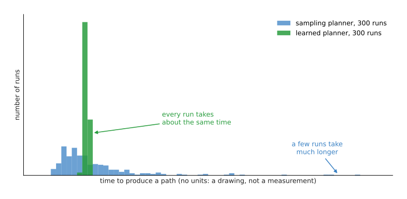
The picture is a drawing of the idea, and not a measurement. The blue bars show a sampling planner, where most runs are quick but a few take much longer. The green bars show a learned planner, where every run takes about the same short time.
For example, a new taxi driver in a city uses a map and works out each route, while an experienced driver has driven thousands of routes and just knows which way to go. So the experienced driver is quicker than the new one. But the experienced driver can still make a wrong turn in a street that has changed, and the map can tell them so. A learned planner matches the experienced driver, while the ordinary planner and collision checker match the map, and they are still needed to check the answer.
2. What goes in and what comes out#
Section 1 described one learned helper, but there are three kinds, and they take different inputs and give different outputs. The table below lists them, and you read each row as one kind of helper.
| Kind | What goes in | What comes out | What it replaces |
|---|---|---|---|
| Learned route planner | a 3D picture of the scene, the arm's current joint angles, the goal | the next arm position, or a whole route | the search part of a sampling planner |
| Learned collision checker | a set of joint angles, and the scene | "hit" or "clear", or a distance to the nearest obstacle | the exact geometric test, while searching |
| Learned inverse kinematics | where the gripper should be, and which way it should point | one or many sets of joint angles that put it there | an iterative solver |
A 3D picture of the scene here usually means a point cloud, which is a list of 3D dots on every surface a depth camera sees, and the point cloud models page explains these.
3. How a learned route planner works#
The first row of the table was the learned route planner, and it comes in two main designs. Both of them feed the scene and the goal into a network.
The first design proposes the next point, over and over, and here is how that design goes.
- A part of the network turns the point cloud into a short list of numbers that describes where the obstacles are.
- The network looks at that description, the current arm position and the goal position, and then it suggests the next arm position, which is a short hop towards the goal.
- The arm position moves to that suggestion, and step 2 repeats.
- It stops when the suggestion reaches the goal.
- A classical collision checker tests each hop, and if a hop hits something, then an ordinary planner finds a replacement for just that hop.
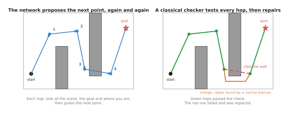
On the left, the network proposes four points in turn, from the start to the goal. On the right, the checker passes the green hops, finds that one red hop clips a wall, and an ordinary planner replaces it with the orange detour.
Step 5 is the important one in that list. The network has learned what good routes usually look like, but it can be wrong, so the check makes sure a wrong route never reaches the arm. And because only one short hop needed repairing, the whole job is still fast.
Two of the models in section 7 work in this way, and they are Motion Policy Networks in sub-section 7.2 and Neural MP in sub-section 7.3. The ordinary planner and the collision checker that step 5 falls back on also have names, and sub-section 7.1 recommends them: MoveIt 2 with OMPL.
The second design is a learned sampler, which keeps the ordinary planner exactly as it is. The only change is where the planner picks its random positions. Instead of spreading them evenly everywhere, a network suggests positions in the places where routes usually pass, such as the gap between two shelves. So the planner finds a route sooner, and it still checks everything itself. No model in section 7 does this, because a learned sampler is code you write against the ordinary planner rather than a file you download, which is what sub-section 7.6 says when it comes to choosing.
4. Learned collision checking#
The second row of the table was the learned collision checker, and it exists because a collision check has to run many thousands of times while a planner searches. Each exact check compares the shapes of every arm link with every obstacle, which takes time. So a learned collision checker is a network that has seen many arm positions labelled "hit" or "clear", and it gives a quick guess for a new position.
Some versions give a distance instead of "hit" or "clear", which is how far the arm is from the nearest obstacle. A distance is useful to planners that improve a route step by step, because it tells them which way to push the route to get further from obstacles.
To see where this goes wrong, think of a simple arm with two joints and a post beside it. Each arm position is just two angles, so you can draw every possible position as one dot on a flat chart. Then the positions where the arm touches the post form a grey region on that chart.
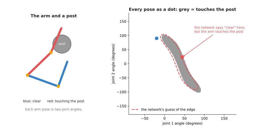
The left picture shows two arm positions, one clear and one touching the post. The right picture shows every position as a dot on a chart of the two joint angles, where the grey region is where the arm touches the post. The red dashed line is the network's guess of that region's edge. It is close, but not exact, so the red dot sits in a place where the network says "clear" when the arm is really touching.
The network is almost always right far from the edge, and its mistakes are near the edge. But that is exactly where a planner spends its time when it squeezes through a gap. So a learned checker is used only to guide the search, and the exact checker still tests the final route. The one published model of this kind is SceneCollisionNet, in sub-section 7.4, and it is kept there as the clearest example rather than as a recommendation.
5. Learned inverse kinematics#
The third row of the table was learned inverse kinematics, and this section says what that sum is. Inverse kinematics, often shortened to IK, is the sum that answers "which joint angles put the gripper here, pointing this way?". The ordinary way to solve it is to start from a guess and improve it step by step, which is quick for easy targets. But it can be slow or fail for awkward ones, and the answer you get depends on the starting guess.
Many arms also have more than one correct answer for the same target. An arm with seven joints, or a flat arm with three joints reaching a point, can reach that target in many different ways, because it can hold its elbow high or low, for example.
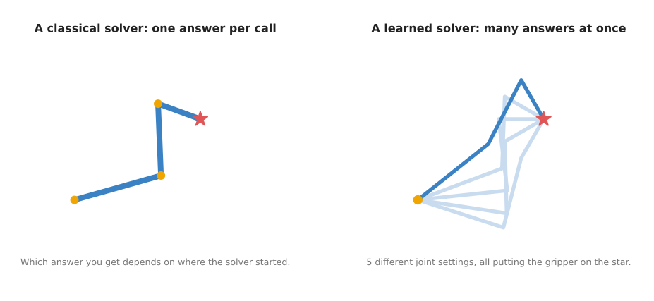
On the left, a classical solver gives one answer. On the right, a learned solver gives five different arm poses at once, all putting the gripper on the red star.
A learned IK solver is a network trained on many pairs of joint angles and the gripper positions they produce. The pairs are easy to make, because you pick random joint angles and work out where the gripper ends up, using the arm's known sizes. That sum, from angles to gripper position, is called forward kinematics, and it is exact and fast, so the network only has to learn to go the other way. Some learned solvers, such as IKFlow, which sub-section 7.5 recommends, give many different answers at once, drawn from all the ways the arm can reach the target. A planner can then choose the answer that avoids obstacles or stays far from joint limits.
But the learned answer is usually close rather than exact. So people pass it to the ordinary solver as a starting guess, and the ordinary solver then finishes the job in a step or two.
6. How they are trained#
Sections 3 to 5 described three different networks, and all three are trained in the same basic way. That way has one large advantage, because the training data is made by a computer, and not collected by people.
- Make many scenes. A program places random boxes, shelves and tables around a simulated arm.
- Ask the slow, correct method. An ordinary planner finds a route in each scene, or an exact collision checker labels many arm positions, or forward kinematics works out gripper positions for many random joint angles.
- Save the questions and answers. Each scene and goal is a question, and the planner's route is the answer to it.
- Train the network to give the same answers. Show it a question, compare its answer with the saved one, and adjust it a little. Then repeat that many times.
Because a computer makes the data, people can make a great deal of it. Motion Policy Networks, which sub-section 7.2 covers, learned from millions of planner answers, so the cost here is computing time, and not human time.
But there is a catch in step 1, because the network only learns scenes like the ones the program made. If the program made boxes on tables, then a real kitchen with a hanging lamp may confuse it.
7. Well-known models of this kind#
Section 6 described how these networks are trained, and this section names the tools you can download and says which one to reach for. It starts with the written planner rather than with a network, because the written planner is what every learned helper here has to beat, and for most moves through open space it still wins.
Read the table one row at a time. The left column names the tool and says how
current it is. The right column holds the rest: what the tool is best at, how
large the download is, its licence, and when to pick it. Where a size is given,
it is the size of the file you have to download, and not a count of the
network's parameters, because these projects publish a trained file and no
parameter count. That file
is called a checkpoint, and it holds the numbers that a training run
produced. Where a row says not stated, the project does not publish that
figure.
| Tool | What decides it |
|---|---|
| MoveIt 2 with OMPL, most used in 2026 | This one is written rather than learned, and it handles any move through open space. It checks every move it gives you against the real shapes. There are no weights to download, and the licence is BSD 3-Clause. Always try this first. |
| cuRobo, most used in 2026 | This one is written rather than learned, and it produces many plans a second, so the arm can react while obstacles move. There are no weights to download, and the licence is Apache-2.0. Pick it when you have an NVIDIA graphics card and the scene keeps changing. |
| Motion Policy Networks, historical | This one gives one route straight from a depth camera, on a Franka arm. Its checkpoint is 229 MB. Its code is MIT, and the checkpoint on Zenodo is Creative Commons Attribution 4.0. Pick it when you want to study how a learned route planner is built and trained. |
| Neural MP, worth betting on | This one does the same job as Motion Policy Networks, and its weights download in one line. Its checkpoint is 86 MB. Its licence is not stated in the code repository, and the weights are tagged MIT. Pick it when you have a Franka arm, an NVIDIA card and a point cloud of the scene. |
| SceneCollisionNet, historical | This one guesses quickly whether a moved object hits anything. Its download size is not stated, and its NVIDIA Source Code License allows non-commercial use only. Pick it for research on tidying a cluttered table. |
| IKFlow, most used in 2026 | This one gives many different joint-angle answers for one gripper pose, and it is the most used of the learned helpers here. The Franka model is 204 MB. Its licence is not stated, because the licence file holds only the text #TODO. Pick it when a seven-joint arm needs a choice of inverse kinematics answers. |
7.1 MoveIt 2 with OMPL, and cuRobo, which are written and not learned#
These two are most used in 2026, because a developer who has to move an arm across a table today installs one of them and not a network.
Neither has a size, because neither is learned and there are no weights to download. MoveIt 2 with OMPL runs on a laptop and is BSD 3-Clause, and cuRobo needs a small card and is Apache-2.0.
MoveIt 2 is the motion planning framework for ROS 2, and it is the one this repository uses. It does not plan by itself. It calls OMPL, a library from Rice University that holds the sampling-based planners section 1 described, and RRT-Connect is the planner it uses when nothing else is configured. cuRobo is a different written planner, from NVIDIA. It tries thousands of candidate trajectories at the same time on a graphics card, which makes it fast enough to plan again every control cycle rather than once per move.
The one idea these two share is that they refuse to guess. Both look for a route in the space of the arm's own joint angles, and both test what they find against the real shapes of the arm and the obstacles before they hand it back. What separates them is how each one copes with the size of that space. OMPL tries one random arm position at a time and keeps the ones that worked. cuRobo never looks at single positions at all: its unit of work is a whole route from start to goal, and it improves thousands of whole routes at the same time on the graphics card.
Inside OMPL, RRT-Connect grows two trees of arm positions, one from the start and one from the goal. Each round picks a random set of joint angles, finds the position already in a tree that is nearest to it, takes one short step from there towards it, and asks the collision checker whether that step is clear. The trees grow until a step from one of them reaches the other, and the route is then the path through the joined trees. Nothing in that loop has a fixed length, because how many random picks it takes depends on luck and on how narrow the gap is. cuRobo's loop has a different shape. It starts from many complete candidate routes, which its paper calls seeds, scores all of them against the obstacles together on the graphics card, and then improves all of them at once: first with a particle-based solver, which carries a cloud of slightly different candidates and pulls the whole cloud towards the better ones, and then with L-BFGS, an optimiser that reads the slope of the score and takes a well-aimed step down it. A separate geometric planner supplies fresh seeds when the candidates it began with all end up stuck.
What OMPL's design buys is correctness and generality. It will plan for any arm
and any set of obstacles, and a route that comes back has been checked step by
step. What it costs is that the time is not bounded: a run that usually answers
in 50 milliseconds will sometimes take a second, because a random search has no
fixed length, and that is the fault that sends people looking at the learned
planners below. What cuRobo's design buys is steadiness, because the same
arithmetic runs on every attempt, so the answers arrive in similar times and the
planner can be called again every control cycle instead of once per move. What it
costs is that an optimiser can settle into a route that is good nearby and silly
overall, so it needs several seeds and can still come back with nothing, which is
why the example below checks result.success.
The difference between the two shows up on a cell that has to hold a cycle time. If the arm has four seconds to move and OMPL answers in 50 milliseconds nine times out of ten and in a second on the tenth, then one part in ten takes longer than planned, and nobody can say which one. cuRobo's planning time varies far less, so the budget holds. The other case is an obstacle that moves while the arm is travelling, such as a person reaching across the table. OMPL planned the route before the person arrived and will not notice; cuRobo can plan the whole route again from the newest obstacles inside one control cycle.
Why pick these rather than any network on this page? Because they check every move they give you against the real shapes of the arm and the obstacles, so a route that comes back has been tested rather than guessed. Every learned planner below is trained on routes that one of these produced, so at best it copies them, and speed is the only thing it can beat them at. You add a network when these two are too slow in a way that costs you money, and not before.
What they cost you beyond the line above is the installation. cuRobo needs CUDA, which means an NVIDIA graphics card, so it does not run on an Apple Silicon Mac at all. And neither is a small install, because MoveIt brings the whole of ROS 2 and cuRobo brings PyTorch and a CUDA toolchain.
The library for the written planner on a graphics card is cuRobo itself, and the code below is shortened from the motion generation example in its documentation.
import torch
from curobo.types.math import Pose
from curobo.types.robot import JointState
from curobo.wrap.reacher.motion_gen import MotionGen, MotionGenConfig, MotionGenPlanConfig

# the world here is one box, 5 m across and 0.2 m thick, standing for the table
world = {"cuboid": {"table": {"dims": [5.0, 5.0, 0.2], "pose": [0, 0, -0.1, 1, 0, 0, 0]}}}

# "ur5e.yml" is an arm description that ships inside cuRobo
config = MotionGenConfig.load_from_robot_config("ur5e.yml", world, interpolation_dt=0.01)
motion_gen = MotionGen(config)
motion_gen.warmup()  # compiles the GPU work once, so later plans are fast

goal = Pose.from_list([-0.4, 0.0, 0.4, 1.0, 0.0, 0.0, 0.0])  # x, y, z then w, x, y, z
start = JointState.from_position(
    torch.zeros(1, 6).cuda(),  # all six joints at zero
    joint_names=["shoulder_pan_joint", "shoulder_lift_joint", "elbow_joint",
                 "wrist_1_joint", "wrist_2_joint", "wrist_3_joint"],
)
result = motion_gen.plan_single(start, goal, MotionGenPlanConfig(max_attempts=1))
print(result.success)
trajectory = result.get_interpolated_plan()
What cuRobo supplies is the collision checking, the inverse kinematics and the
optimisation, all on the graphics card, and descriptions of several arms. What
you supply is the world: the box above stands for a table, and on a real cell you
replace it with the obstacles your depth camera reports, which is the part that
takes the time. You also have to check result.success, because the planner can
fail and the answer is then not a trajectory.
7.2 Motion Policy Networks, which showed that the idea works#
This one is historical, kept because it is the clearest example of how a learned route planner is built, and because the model after it is built the same way.
Size not stated, and the checkpoint is a 229 MB download. A small card. MIT for the code, and Creative Commons Attribution 4.0 for the checkpoint, which is a different licence on the part you actually run.
Motion Policy Networks, often written MPiNets, is NVIDIA's learned route planner from 2022, published at the Conference on Robot Learning. It takes a point cloud and a goal pose for a Franka arm, and it proposes the next arm position over and over, which is the first design from section 3. Its predecessor was MPNet, from the University of California, San Diego, in 2019, which had the same idea and has not been changed since 2020.
The one idea behind MPiNets is that a route does not have to be searched for. It can be a habit. The network is given what the camera sees now, the arm's current joint angles and the goal, and it answers with the next small movement in one pass. Repeat that pass and you have a route. So where sub-section 7.1 asked a question and waited for a search to finish, this asks a question and gets an answer in a known amount of arithmetic.
What that changes inside is that the two trees and the random picks are gone, and two pieces stand in their place. The first reads the point cloud. The repository's loop hands it 2048 points sampled on the arm's own surface, then the points the camera saw on the obstacles, then points on the target, with each group marked so the network knows which is which, and it turns all of that into a short list of numbers. The second piece reads that list together with the seven joint angles, rescaled to the range from minus one to one, and returns a step to add to those angles rather than a position to travel to. The new angles are then used to redraw the arm's own points in the point cloud, and the loop runs again. Notice what is not in that loop: the collision checker, which inside OMPL was consulted on every single step, is not consulted here at all.
What the idea buys is that the cost of an answer no longer depends on the
problem, because the loop in the code below runs a fixed number of passes and
then gives up. What it costs comes in two parts. Nothing inside the loop knows
whether a step hits anything, so a wrong step reaches the arm unless you test the
finished route yourself, which is step 5 of section 3. And the network only knows
the kinds of scene its teacher solved. That teacher was the real contribution of
the paper: a planner made to answer the same problem the same way every time,
because a network cannot copy a teacher who gives a different route on each
asking, and a random planner does exactly that. The checkpoint file is named after
that teacher, mpinets_hybrid_expert.ckpt.
The difference shows up when the scene changes during a move. If a box is set down beside the arm after the move has started, MPiNets takes the newest point cloud and gives the next step at exactly the cost of the first one, where RRT-Connect has to throw away its trees and search again from where the arm now is. The difference runs the other way as soon as the scene stops looking like a table with boxes on it. Hang a lamp over the table and MPiNets can propose a step straight through it, while OMPL, which asks the real shapes rather than remembering, simply reports that the step is blocked.
Why pick it rather than Neural MP, which is newer and comes next? Only for reading and reproducing. MPiNets publishes the whole pipeline that generated its training data, which is the part of the work that a team building its own learned planner actually needs, and its code is MIT. Its code was last changed in 2023, so for running an arm the newer model is the better choice.
What it costs you is the installation. The recommended way to install it is a
Docker container of about 30 GB, built on top of NVIDIA Isaac Sim, and building
that container needs an NVIDIA developer account. There is nothing to pip install, and the thing that most often goes wrong is the installation rather
than the model.
The library is the repository's own mpinets package. The lines below are
shortened from rollout_until_success in
its inference script,
and they are the whole of what the network does.
import torch
from mpinets.model import MotionPolicyNetwork
from mpinets.utils import normalize_franka_joints, unnormalize_franka_joints

model = MotionPolicyNetwork.load_from_checkpoint("mpinets_hybrid_expert.ckpt").cuda()
model.eval()

trajectory = []
q_norm = normalize_franka_joints(q)  # the seven joint angles, rescaled to -1 to 1
for _ in range(150):  # the script's own limit, after which it gives up
    # the network returns a step to add to the current position, not the position itself
    q_norm = torch.clamp(q_norm + model(point_cloud, q_norm), min=-1, max=1)
    trajectory.append(unnormalize_franka_joints(q_norm))
    # the script stops here once the gripper is within 1 cm and 15 degrees of the
    # target, and the point cloud's robot points are redrawn for the new position
The repository supplies the trained network, the point cloud handling and a measurement script. What you supply is the checkpoint, a 229 MB download from Zenodo, and the point cloud in the exact form the network expects, which is 2048 points sampled on the arm's own surface followed by the obstacle points and the target points. You also supply the collision check on the result, because nothing in the loop above tests whether a step hits anything.
7.3 Neural MP, the same idea with weights on Hugging Face#
This one is worth betting on, because it is where the published work is going: it ships its weights in the ordinary Hugging Face way rather than as a file beside a paper, and its own authors have already published a follow-up aimed at obstacles that move.
Size not stated, and the checkpoint is an 86 MB download. A small card, on Linux. No licence at all in the code repository, and an MIT tag on the weights.
Neural MP comes from Carnegie Mellon University and was published at the 2025 conference on intelligent robots and systems. It is the same kind of network as MPiNets, taking a point cloud and proposing joint positions, and it adds a short optimisation at the end to repair the route it proposed. Its own follow-up is Deep Reactive Policy, from 2025, which aims at scenes where obstacles move while the arm is moving.
Neural MP keeps MPiNets' one idea and changes two things about it. Its paper's claim is a large number of complicated scenes built in simulation, which pushes back the catch section 6 described without removing it: the more kinds of scene the program made, the fewer real rooms are unlike anything the network has seen. And the repair of the proposed route is part of the tool instead of being your job.
Inside, the first difference you meet is not in the network but in what you are
asked for. MPiNets takes a goal pose, meaning a place in the room and a direction
to point in, and works out the joint angles itself. Neural MP takes
goal_config, which is the seven goal joint angles, so the choice of which way to
hold the elbow has already been made before the model is called, by an inverse
kinematics solver such as the one in sub-section 7.5. The second difference comes
after the proposal. motion_plan_with_tto takes the whole route the network
proposed and runs a short optimisation over it, pushing it away from the points
the cameras reported, which is the step MPiNets leaves to an outside planner. The
network's own loop is otherwise the same shape: a point cloud, the current joint
angles, a step, repeat.
What that buys is a route that has already been pushed off the obstacles, from a
starting point the network believes in. This is also the honest difference from
cuRobo, which optimises too. cuRobo's optimiser begins from seeds that may be far
from any sensible route, so on a hard scene it needs more attempts, while Neural
MP's optimiser begins from a route the network already thinks is good and has less
to do. What it costs is that the repair is a second, slower pass, so the promise
of a fixed number of network calls holds for motion_plan and not for
motion_plan_with_tto. And asking for joint angles rather than a pose means you
owe the model an inverse kinematics answer, and a rule for choosing among the
several answers an arm with seven joints has.
The difference shows up when the route has to hug an obstacle. Reaching into a cubby, where the gripper must travel between a shelf and the box above it, MPiNets hands you a route near the shelf and leaves you to notice that one hop clips it. Neural MP's own optimisation pushes that route off the shelf before you see it. The difference runs the other way when the goal is naturally a pose, as in "put the gripper here, pointing down": MPiNets takes that directly, and with Neural MP you have to solve for the joint angles first.
Why pick it rather than MPiNets? Because the weights come down in one line, with
from_pretrained, from a Hugging Face
repository where the checkpoint is a
single 86 MB file tagged MIT, and because its code was last changed in 2026 where
MPiNets was last changed in 2023. Why pick it rather than cuRobo, which also runs
on a graphics card? Because it answers in a fixed number of network calls, where
cuRobo's optimiser can need more attempts on a hard scene. If neither reason
applies, cuRobo is less work.
What it costs you is a Linux machine with an NVIDIA card, and its tested configuration is Python 3.8 with CUDA 12.1. The code repository has no licence file at all, which is not the same as being free to use, even though the weights on Hugging Face carry an MIT tag. The thing that most often goes wrong is the point cloud, because the model expects 2048 points on the arm and 4096 on the obstacles, and badly calibrated cameras plan a route around obstacles that are not where the model thinks they are.
The library is the repository's own neural_mp package, and the planner is one
method call.
from neural_mp.real_utils.neural_motion_planner import NeuralMP

planner = NeuralMP(env=env, model_url="mihdalal/NeuralMP", train_mode=False, in_hand=False)

# points and colors are the combined point cloud from your calibrated cameras
trajectory, success, mean_time = planner.motion_plan(
    start_config=start_joint_angles,   # seven joint angles
    goal_config=goal_joint_angles,     # seven joint angles, not a gripper pose
    points=points,
    colors=colors,
)
What the library supplies is the trained network, the point cloud preparation and
the rollout, and motion_plan_with_tto runs the repair step as well, more slowly.
What you supply is env, a wrapper around your own Franka control code, and the
cameras behind points. The important detail is goal_config: Neural MP plans
from joint angles to joint angles, so a gripper pose has to be turned into joint
angles first, which is what section 7.5 is for.
7.4 SceneCollisionNet, which learns the collision check#
This one is historical. It is the clearest published example of a learned collision checker, and it has not been changed since 2021.
Size not stated, and no download size is published either, because the weights arrive through a script. A small card. The NVIDIA Source Code License, for the code and the weights alike, which allows non-commercial use only.
SceneCollisionNet came from NVIDIA and the University of California, Berkeley, in 2021. It takes a point cloud of a scene and a pose for an object, and it says quickly whether the object in that pose would hit anything, which is the second row of section 2's table. It was built to plan where to put objects down when tidying a cluttered table. The other well-known approach is Fastron, from the University of California, San Diego, which is C++ code that builds a quick collision guesser for one arm and updates it as obstacles move.
The one idea here is easy to miss, because it is not speed. It is that the question is asked about things that have no shapes on file. An exact collision checker compares one mesh with another, and a mesh is a list of triangles describing a surface, so it can only answer about objects somebody has modelled. SceneCollisionNet is asked instead about a scene that is a cloud of points from a depth camera, and an object that is another cloud of points, neither of which has ever been modelled. The exact checker can still be given a crude box drawn around those points, but a box is either larger than the object, so it refuses places the object would have fitted, or wrong on the side the camera could not see. The paper makes that its case: the learned model is for the times when a model of the object is not available.
What that changes inside is that the question is split into a part that is asked once and a part that is asked many times. One encoder reads the scene's point cloud and keeps a description of it. A second encoder reads the points of the object now in the gripper. Then, for each pose you are considering putting that object in, a small network reads both descriptions and answers "hit" or "clear". Because the scene description is computed once and reused, thousands of candidate poses are answered together in one go on the graphics card. The learned planners above read a point cloud too, but they read it in order to produce a movement; this one reads it in order to answer a question about a movement somebody else proposed.
What the idea buys is that "where can I put this down?" becomes one batch of answers instead of thousands of separate comparisons, and it works on objects you have no model of. What it costs is the thing section 4 drew: the guess is wrong near the edge of an obstacle, and near the edge is exactly where a good place to put something down tends to be. So the paper used it to score and rank many candidate placements inside a controller, and not as the last word before the arm moved.
The difference shows up on a table of objects nobody has modelled. You pick up an unfamiliar jar and want to know which of three hundred free spots it will fit in. MoveIt's exact checker has to stand in a box for the jar and another for each piece of clutter, and the answer it then gives is exact about the boxes and not about the things. Ask the opposite question, "does this arm configuration collide?", and MoveIt wins outright, because the arm's own shapes are known exactly and the answer is then right rather than probable.
Why pick it rather than the exact collision checker inside MoveIt? Only when you have to test very many poses and that test is what is holding you up, as when you score hundreds of candidate places to put an object down. For the ordinary question of whether one arm position collides, the exact check is correct and quicker to set up, and section 4 explained that a learned checker is wrong exactly at the edge of an obstacle, where a planner spends its time.
What it costs you is the licence. The repository carries the NVIDIA Source Code License for SceneCollisionNet as a PDF rather than as a standard licence file, and section 3.3 of that licence limits the work and anything derived from it to non-commercial use. So you can study it and you cannot ship it. The code is also from 2021 and expects CUDA 10.2.
The library is the repository's own scenecollisionnet package, and the useful
thing to run is its own comparison of the learned checker against the exact one.
Both commands come from its README.
bash scripts/download_weights.sh                     # the trained networks

# the learned checker, then the exact checks it is compared against, which are
# FCL, the Flexible Collision Library, and a signed distance field
PYOPENGL_PLATFORM=egl python tools/benchmark_scenecollisionnet.py
PYOPENGL_PLATFORM=egl python tools/benchmark_baseline.py
What the repository supplies is the trained networks and that comparison, so you can see the trade for yourself. What you supply is the mesh dataset, which its README builds from ShapeNetSem meshes and the ACRONYM grasp set.
7.5 IKFlow, which gives many inverse kinematics answers at once#
Of the learned helpers on this page, this is the one that is most used in 2026, because it is the only one that installs on an ordinary Linux machine and ships trained weights for several named arms.
Size not stated, and the Franka Panda model is a 204 MB download. A small card,
and it falls back to the processor when there is none. No licence at all, because
the licence file holds only the text #TODO.
IKFlow is a learned inverse kinematics solver from the paper IKFlow: Generating Diverse Inverse Kinematics Solutions, published in 2022. It is the model section 5 described: you give it a gripper pose, and it returns many different sets of joint angles that all reach that pose. The repository publishes trained models for the Franka Panda, the Fetch arm and the Rizon 4.
The one idea here is that the network learns the whole set of answers rather than one answer. The repository describes itself in a single line as normalizing flows for inverse kinematics, and a normalizing flow is a network built so that it can be run in both directions with one set of weights. Training teaches it to turn real answers into plain random numbers, and using it means running it backwards, turning fresh random numbers into real answers.
That is a different shape of network from every other model on this page, and the difference matters most in what it avoids. The learned models above are all trained to produce one output for one input, which is fine when there is one right answer. Inverse kinematics is not like that: an arm with seven joints reaches most poses with the elbow high or with the elbow low. A network trained to give one answer is pushed towards the middle of those two, and the middle of two valid arm poses is usually not a valid pose at all. IKFlow is never asked for the middle. You hand it the target pose and a fresh set of random numbers, and it runs backwards to one set of joint angles. Hand it five different sets of random numbers and the same pose, and five different arm poses come back, each a real way of reaching the target.
What the idea buys is a choice, which the written solver cannot offer at any price, and all of the options in a single pass. What it costs is exactness. The answers are near the target rather than on it, so you finish them with the ordinary numerical solver, which is the last line of the example below. You also owe the model the rule for choosing, because a spread of answers is useless until something decides between them. And the arm's own sizes are baked into the trained weights, so a new arm means a training run of your own rather than a new configuration file.
The difference shows up on a seven-joint arm reaching into a shelf. The ordinary
solver returns whichever answer its starting guess led to, and if that answer puts
the elbow through the shelf, your only recourse is to change the guess and hope.
IKFlow hands you a dozen answers for the same pose, you run the exact collision
check over all of them, and you keep one that is clear. This is also how a gripper
pose becomes the goal_config that Neural MP in sub-section 7.3 demands.
Why pick it rather than the numerical solver that MoveIt already calls? Because the numerical solver returns one answer, and which one depends on the guess it started from. An arm with seven joints can reach almost any pose in many ways, and you often want to choose among them, taking the answer furthest from the joint limits or nearest to where the arm already is. IKFlow gives you a spread of answers in one pass, and the written solver cannot do that at all. If one answer is enough, use the written solver.
What it costs you is a careful installation. The README says the only supported
operating system is Ubuntu, and it installs from a clone of the repository with
uv sync rather than from the package index, where the latest ikflow release is
version 0.0.8 from February 2023 and far behind the repository. Since the licence
file says only #TODO, no licence has been granted, which is a question to settle
before a product. The thing that most often goes wrong is forgetting that the
answers are approximate, and the next is the quaternion order, which is
w, x, y, z here and the other way round in several other libraries.
The library is ikflow, and the code below asks for five answers to one pose.
import torch
from ikflow.model_loading import get_ik_solver

# the name must match an entry in ikflow/model_descriptions.yaml; this one
# downloads a 204 MB trained model for the Franka Panda
ik_solver, _ = get_ik_solver("panda__full__lp191_5.25m")

# x, y, z in metres, then a rotation as a quaternion in the order w, x, y, z
target_pose = torch.tensor([0.5, 0.5, 0.5, 1.0, 0.0, 0.0, 0.0])

# five different sets of joint angles, all reaching about the same pose
solutions = ik_solver.generate_ik_solutions(target_pose, n=5)

# the same five, finished off by an ordinary numerical solver
exact, _ = ik_solver.generate_exact_ik_solutions(target_pose.expand((5, 7)))
What the library supplies is the trained models, the sampling, and the polishing
step in the last line, which runs ordinary numerical steps on the network's
answers. The repository's own benchmark calls those polished answers exact to
within 1 mm and 0.572 degrees, and the answers from generate_ik_solutions are
not. Passing return_detailed=True also tells you which answers break a joint
limit or make the arm touch itself. What you supply is your arm, if it is not one
of the published ones, which means its description file and a training run of
your own. You also supply the rule for choosing among the answers, because the
model has no opinion about that: the answer nearest the current joint angles
avoids a large sudden movement, while the answer furthest from the limits leaves
more room for the move after it.
7.6 How to choose#
Start with MoveIt 2 and OMPL, and add nothing learned. That is the right answer for almost every arm that moves through open space, because the written planner checks what it gives you and costs nothing to train.
Four things change that answer.
If the planning time is usually fine but sometimes far too long, and a cell is waiting on it, then look at the speed first and the learning second. cuRobo on an NVIDIA card removes most of that unevenness with no training at all, and it is less work than any model on this page. Try it before you train anything.
If you need a route in a fixed number of steps on a Franka arm, and cuRobo's optimiser still takes a varying number of attempts, then Neural MP is the learned planner to try, because its weights download in one line. Keep the exact collision check on its answer.
If a seven-joint arm needs several inverse kinematics answers to choose from, then IKFlow is the one tool here that does something the written solver cannot do at all. Settle its licence first.
If you are building your own learned helper rather than using one, read Motion Policy Networks, because it publishes the pipeline that generated its training data. A learned sampler of the kind section 3 described is code you write against OMPL, and not a model you download.
One case needs no planner at all. If the part is always in the same place, teach the route once and play it back.
8. Where this is going#
Section 7 named the tools that exist today, and this section says where this kind of model is heading. Each statement below says what kind of claim it rests on, using the four kinds the frontier chapter sets out, and where a judgement is mine rather than somebody's claim the sentence says so.
8.1 How it got here#
Every learned helper on this page grew out of one complaint, which is that a sampling planner's running time has no upper bound. Motion Policy Networks answered it in 2022 by learning a planner's answers, and Neural MP repeated the answer in 2025 with weights you can download in one line. What happened beside them is the part a reader usually misses. The written planners did not stand still. They moved onto the graphics card, and they got there first, so the same complaint was being answered from both directions at once.
8.2 Where it is used in industry today#
A learned planner is almost absent from industry, and that is the honest summary rather than a hedge. I could find no product announcement from any vendor saying that a neural network plans the route of an arm you can buy. What industry buys instead is written planning, sold as a supported product, and it is worth naming because it is what a learned planner would have to displace.
PickNik Robotics sells MoveIt Pro and MoveIt Pro Core, the commercial build of the MoveIt 2 stack from sub-section 7.1, and its own customer pages name NASA's Johnson Space Center, the BMW Group, Lockheed Martin and Philips. On 23 September 2026 Qualcomm announced that it will acquire PickNik and stated that MoveIt 1 and MoveIt 2 will "remain open, community-driven, and supported across third-party hardware platforms". The acquisition had not completed when this was written, so the promise about openness is still a projection. A chip vendor paying for the motion planning layer is the clearest available signal about where the money in this area sits.
Realtime Robotics sells Resolver and RapidPlan, and its business is planning and deconflicting the routes of several arms sharing one cell. Its own pages name Daimler Truck, Mercedes-Benz, Schaeffler, KUKA, FFT, EDAG and Valiant TMS as customers, and describe one application at FFT with 120,000 weld points and four robots. Those figures come from vendor marketing, so read them as a product announcement about what the software is sold to do rather than as a measured result. NVIDIA ships cuRobo into ROS 2 as isaac_ros_cumotion, so the written graphics-card planner installs as an ordinary MoveIt planning plugin. That one is a download you can check today.
8.3 What is being worked on right now#
The most consequential current work is not on the learned side at all. cuRoboV2, by Balakumar Sundaralingam, Adithyavairavan Murali and Stan Birchfield, appeared on 5 March 2026 and shipped in NVIDIA's own repository as cuRobo v0.8.0 under Apache-2.0 on 18 April 2026. The paper reports 99.7 per cent success under a 3 kg payload where its baselines reach 72 to 77 per cent, 99.6 per cent collision-free inverse kinematics on a 48-joint humanoid, and up to a 61-fold speedup in whole-body computation. Those are research results whose code is a download, which is an unusually strong pairing. Read the inverse kinematics figure next to sub-section 7.5: a written solver now reports 99.6 per cent collision-free answers on a body far larger than a Franka arm, and that is the number a learned solver now has to beat.
The learned side's own front has moved to scenes that change while the arm is moving. The clearest result is Deep Reactive Policy from Carnegie Mellon University, published at the 2025 Conference on Robot Learning as arXiv 2509.06953. Its core, called IMPACT, is a transformer trained on 10 million generated planner trajectories, and it reads a point cloud directly. The project's own page reports success rates against both cuRobo and Neural MP, and the shape of them is the useful part. In static scenes it reports 84.6 per cent against cuRobo's 82.97 per cent, which is a tie. On obstacles that appear suddenly it reports 86 per cent against 59. On goal blocking, where something sits on the place the arm was told to reach, it reports 66.67 per cent against 0 for cuRobo and 0 for Neural MP. These are research results from the authors' own page, which marked the code as a pre-release when this was written, so nothing here is a product announcement yet.
The pattern in those three rows is the thing to carry away. A learned planner does not win by being quicker at the job cuRobo already does well. It wins by scoring above zero where the written planner cannot start, which today means a world that moves.
Diffusion models are the other active line. Motion Planning Diffusion learns a distribution over whole trajectories and steers the sampling with a cost, so avoiding obstacles becomes a nudge during generation rather than a hard test. Work in 2026 uses the same generator for the starting guess of an ordinary optimiser instead of for the final answer, as in warm-starting collision-free model predictive control. I expect the second use to last, for the reason in sub-section 7.3: a proposal that an exact method then repairs only has to be roughly right, so its mistakes cost time rather than safety.
The field has also begun writing down its own open problems. Toward Generalist Neural Motion Planners for Robotic Manipulators, from 25 March 2026, is a survey whose stated finding is that current neural motion planners "often struggle to generalize to unseen, out-of-distribution planning settings". A survey still naming generalisation as the obstacle, four years after Motion Policy Networks, tells you more than any single success rate.
8.4 What is still unsolved#
A learned planner cannot tell you that no route exists. A sampling planner is probabilistically complete, which means it will find a route if one exists and it is given enough time, so a long search returning nothing is at least weak evidence that the gap is too tight. A network returns an answer of the same shape whether the problem is solvable or not, and nothing in that answer separates a route from a confident guess at a route that is not there. Nobody has published a learned planner that reports its own failure reliably, which is why every system in this section keeps a written collision checker downstream.
Generalisation beyond the scene generator is the second, and section 6 named the mechanism. The training scenes are made by a program, so the network learns that program's idea of a room. Neural MP's answer was to generate far more kinds of scene, which pushes the boundary back without removing it, and the 2026 survey above reports that the boundary is still the open problem.
The third is mundane and it stops real projects. IKFlow's licence file holds only
the text #TODO, Neural MP's repository states no licence at all, and
SceneCollisionNet's forbids commercial use, so the three most interesting learned
helpers here grant you no clear rights over the part you run. OMPL and cuRobo have
no such problem.
8.5 The next two to three years#
Everything in this sub-section is my own expectation unless the sentence names somebody else's commitment.
I expect the learned route planner to lose ground rather than gain it, because written code now supplies the one advantage it had. Its case was always a short answer time that does not vary. cuRobo's design gives that without any training, its version 2 is a download under Apache-2.0, and NVIDIA ships it into ROS 2. When the written tool is predictable, free, checked against the real shapes and now paid for by chip vendors, a network has to be better and not merely faster. That is my judgement, not an announcement by anybody.
I expect the learned pieces that survive to be the ones doing something written code cannot do at all, and learned inverse kinematics is the clear case. A numerical solver gives one answer. IKFlow gives as many as you ask for from one gripper pose, and sub-section 7.5 explains why the average of two valid arm poses is usually invalid, so this is a difference in kind and not in speed. CppFlow, by IKFlow's own author and published at the 2024 International Conference on Robotics and Automation, already uses those many answers to plan a Cartesian path, which is a path where the gripper follows a line through space. It is MIT licensed, which the model it builds on is not. I expect that shape to spread: the network supplies the variety, and a written method picks from it and checks the pick.
I expect reactive planning to be where the two approaches actually meet, and Deep Reactive Policy's numbers are the reason. A written planner that replans every cycle still plans against the obstacles it can see, so an obstacle sitting on the goal leaves it nothing to plan towards, which is why cuRobo scores 0 on that row. A network trained on millions of scenes will propose something anyway, and a proposal a checker can reject is worth more than no proposal. So I expect the learned part to settle into the proposal step inside a written planner rather than replacing it. Neural MP's trajectory optimisation and the warm-start papers above are both already that shape.
I expect certification to push against learned planning in Europe, and that expectation rests on a date somebody else published. The European Commission's own machinery page states that Regulation (EU) 2023/1230 applies on a mandatory basis from 20 January 2027 and adds provisions for machinery whose safety functions are powered by artificial intelligence. A written planner's answer can be shown to have been tested against the real geometry, one step at a time, and a network's answer cannot be shown to have been tested at all without the checker behind it. I expect this to make that checker permanent rather than to ban anything, because keeping it is cheap and arguing with an assessor is not.
Last, I expect the planner's job to shrink from a direction this page does not cover. A vision-language-action model takes camera images and a sentence and emits motor commands, with no separate motion planner in the path at all, and the frontier chapter on foundation models records what those models can now do. If the short reach to an object gets absorbed into one such policy, what is left for a planner is the long travel through open space, which written planners already handle well. So I expect learned route planning to lose work in both directions, to the graphics-card planner underneath it and to the end-to-end policy above it. What is left over is many-answer inverse kinematics and reacting to a world that moves, which is exactly where the two strongest results of the last two years are.
9. Where to read next#
This page and the previous one both took over one part of an ordinary system. So the reading below either compares them, or it moves on to the two methods that supply data and scores instead.
In this chapter:
- Reinforcement learning policies covers learning by trying, which suits the contact at the end of a move.
- Diffusion and flow policies covers copying a person's movements.
- The movement models overview compares every kind in this chapter.
In other chapters of this book:
- Point cloud models explains how a network reads the 3D dots these planners take in.
- Learned arm models covers networks that learn the arm's own body.
- Collision and failure detection covers noticing a collision that has already happened, which is a different job.
Deeper documents elsewhere in this repository:
- Learned pieces inside a planned system covers the same helpers for a reader who knows planners well.
- Sampling-based planners explains the ordinary planner these networks learn from.
- What collision checking really checks explains the exact check that stays in the system.
- Redundancy, and the seventh joint explains why one gripper target can have many joint answers.