The page before this one, vision-language-action models, ended with an arrangement where a large slow model decides what the arm should aim for, and a small fast one moves the joints towards it. Every model in this chapter so far, including that one, works the same way underneath. It looks at what is in front of it and says what to do next. None of them has any idea what will happen afterwards.
This page is about the models that do have that idea. A world model is a model that predicts what the world will look like after the robot acts, so that the robot can try something out before doing it. The name is used for a whole family of models, from a few numbers predicting a few numbers, up to a model that generates video. Every member of the family has the same job: given what is true now and what the robot is about to do, say what will be true next.
This page is for a reader who has read the three pages before it in this chapter. You should already know what a policy is, what an action chunk is, and why generative models suit actions. You should also have read reinforcement learning, which is where the words state, action and reward are explained, because this page uses them in the same way.
Everything here is measured on one small simulated system. That system is a robot joint
with a motor, with friction, and with a hard stop that it cannot turn past. A learned model
of that joint is fitted from recorded movements and then pushed until it fails. It fails in
three ways, and all three carry over to the much larger models used on real robots. The
error grows as the prediction runs on. Reducing the pictures to a few numbers throws away a
detail that a grasp depends on. And the one event that a recording almost never contains is
the event the model gets most wrong. By the end of the page you will know what a world
model can be trusted to say, for how long it can be trusted, and what it costs to run one.
The script that works all of this out is
docs/diagrams/models_that_act_2.py.
Contents#
- What a learned dynamics model is
- Why the prediction happens in a squeezed-down space
- Error that piles up over a rollout
- Planning against a learned model
- Video prediction and neural simulators
- When the model gets the physics wrong
- Where to read next
- Using it in Python
1. What a learned dynamics model is#
The simplest member of the family is the one to start from, because everything else on this page is a larger version of it. A learned dynamics model is a model that takes what the robot can see now, together with the action it is about to take, and gives back what it will see one step later. The word dynamics means how the state changes over time. The word learned means that the rule was fitted from recordings rather than written out by a person.
The next picture shows one such step on the simulated joint, with the model's answer beside the true answer.
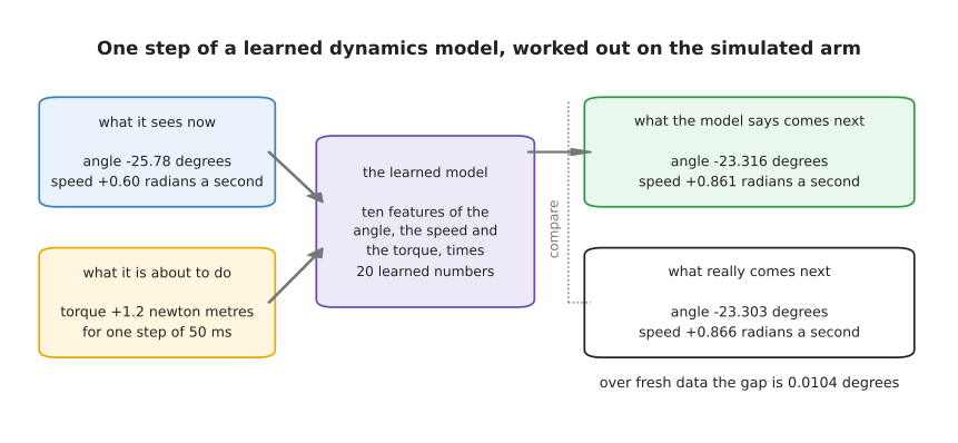
The joint starts at an angle of -25.78 degrees with a speed of +0.60 radians a second. The motor then applies a torque of +1.2 newton metres for one step of 50 milliseconds. A torque is a turning force, and the newton metre is the unit it is measured in. The real joint then reaches -23.303 degrees, and the learned model says -23.316 degrees.
The model is small on purpose, so that nothing is hidden. It takes the angle, the speed and the torque, and works out ten simple combinations of them, such as the angle times the speed. It then multiplies those ten numbers by twenty learned numbers to get the change in angle and the change in speed. Fitting it is one least-squares solve, which means finding the twenty numbers that make the total squared error on the recording as small as possible. On a real robot the same job falls to a network with millions of weights, but the shape of the task is identical.
What the model learns from is a recording of the arm being driven around, of the kind a teleoperated demonstration produces. Teleoperated means that a person drove the arm by hand. The next picture shows where in the recording those movements sit. The two panels measure the same recording in two ways: the scatter shows where the transitions are, and the bars count how many of them reach the hard stop.
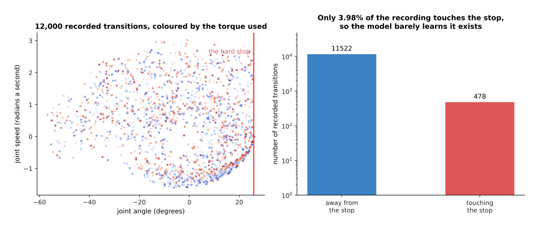
The recording holds 12,000 transitions, and only 478 of them, which is 3.98 per cent, ever touch the hard stop. So that is almost all the model gets to learn about what happens when the arm runs into something.
Those 478 transitions are left out of the fit. That sharpens the point without changing what really happens, because a real recording contains very few collisions for the same reason: the person driving the arm was avoiding them. One step at a time, the fitted model is very good, and the next picture shows how good. Both panels measure the same set of one-step predictions: the left one plots each prediction against the truth, and the right one counts the mistakes.
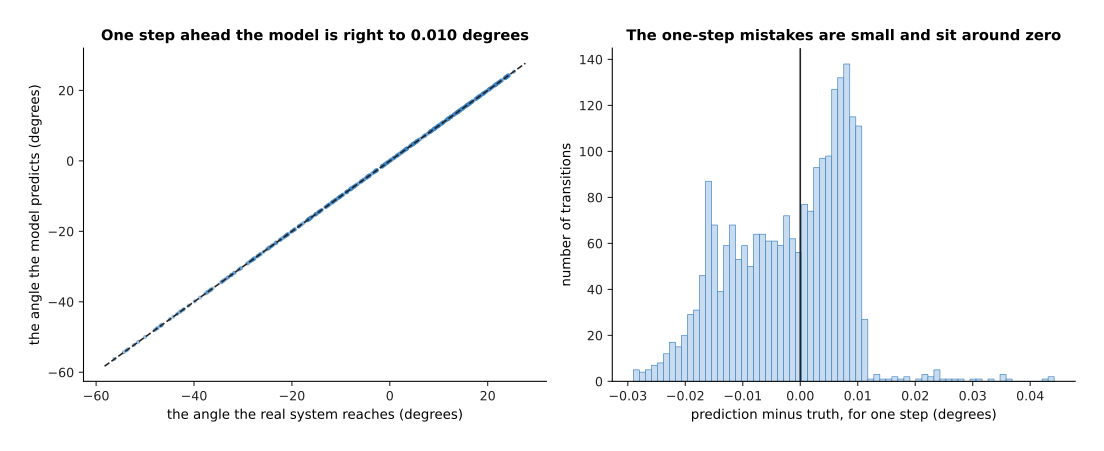
On data it never saw, the model predicts the next angle to within 0.0104 degrees and the next speed to within 0.0033 radians a second.
That is the number that usually gets reported, and on its own it is misleading, which is what section 3 is about. First it is worth seeing what the model actually learned, because the shape of what it got right explains where it will go wrong.
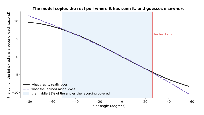
Inside the angles the recording covered, which run from -51.0 to 25.8 degrees, the learned pull on the joint is wrong by 0.0751 radians a second each second. Outside those angles it is wrong by 1.0674, which is fourteen times worse.
Gravity pulls on the joint in proportion to the sine of the angle, and the model has no sine in it, only squares and products. Inside the range it saw, a curve made of squares can be bent to match a sine closely enough. Outside that range nothing holds the two together, so the model's version keeps going down while the real pull flattens off. That is the story of this page in one picture: a learned model copies what it was shown and invents what it was not.
2. Why the prediction happens in a squeezed-down space#
The model in section 1 predicted two numbers from three, which is easy, because the state of that joint really is two numbers. A real robot is not told its state in that form. It gets camera pictures instead, and a camera picture is an enormous list of numbers, most of which have nothing to do with what will happen next.
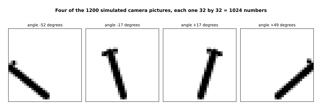
Each of these simulated camera pictures is 32 by 32 pixels, so 1,024 numbers. A modest real camera frame of 256 by 256 pixels in colour is 196,608 numbers.
Predicting all 196,608 numbers of the next frame is an enormous job, and almost all of that work is wasted, because what the robot needs to know is where the arm is and what it is holding. So almost every world model used on a robot first reduces the picture to a short list of numbers, and then predicts the next short list. This page calls that reducing step squeezing the picture down. The short list it produces is called a latent, which means hidden, because those numbers are not anything you can point at in the picture. A model that predicts the next latent rather than the next picture uses latent dynamics. How short the list can be has a measurable answer, and the next picture gives it.
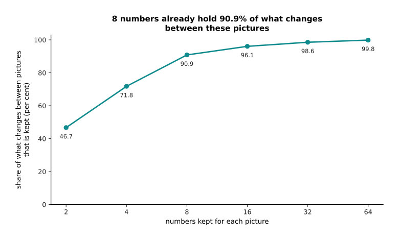
Eight numbers already hold 90.86 per cent of everything that changes between these pictures, and thirty-two numbers hold 98.56 per cent.
The saving that follows is large, because the size of a predictor grows with the square of the number of inputs. The next picture counts the weights for four sizes of state.
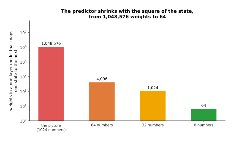
A one-layer predictor over eight numbers needs 64 weights, where one over the raw pixels would need 1,048,576.
The squeezing here uses principal components, which is the simplest method. Principal components finds the directions in which the pictures differ most from each other, and keeps the numbers that say how far along those directions each picture lies. In other words, it keeps whatever varies most across the pictures. Real systems use a trained encoder instead, which is a small network that learns its own short list, but it does the same thing and the sizes come out in the same range. The saving is why nearly every world model on a robot works this way. The cost is that what gets thrown away is chosen by how much it varies, and nothing in that rule knows which parts the robot needs.
The next picture shows the same two camera pictures three times over: as they really are, rebuilt from eight numbers, and rebuilt from sixty-four.
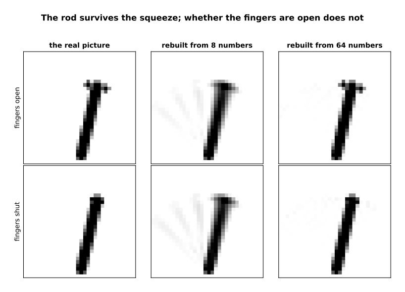
The two real pictures sit at the same rod angle of 12.9 degrees and differ only in whether the fingers are open. Rebuilding them from eight numbers gives the same picture twice.
The rod is large and it moves, so it accounts for most of the variation and it survives the squeeze. The fingers are a few pixels and they only open and shut, so they contribute almost nothing to the variation and they are thrown away. The effect can be measured by asking how often the open or shut state can be read back out of the short list, and the next picture measures it.
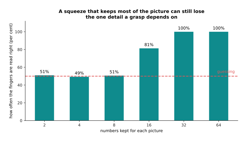
From eight numbers, which hold 90.86 per cent of the picture, whether the fingers are open is read right 50.7 per cent of the time. There are two answers, so 50 per cent is what pure guessing gives. It takes thirty-two numbers before the fingers are read right every time.
That is the honest cost of latent dynamics, and it is not small. A squeeze that looks excellent by the usual measure can be useless for the one decision that matters, because grasping depends entirely on whether the fingers are open. The fix is to stop choosing the latent by how much things vary, and to train it against the job instead. That is why world models for robots are trained together with the policy rather than on their own.
3. Error that piles up over a rollout#
Section 1 ended with a model that predicts one step to within 0.0104 degrees. This section is about what happens when you ask it for more than one step. A rollout is the name for running a model forward repeatedly, feeding its own prediction back in as the next input. It is how any plan longer than one step gets made.
The next picture follows one rollout. Both panels describe the same run: the left one draws the two paths, and the right one draws the gap between them.
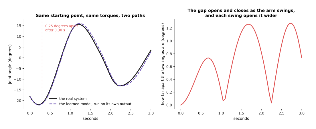
Both runs start from the same state and are given exactly the same torques. The two paths are 0.25 degrees apart after 6 steps, which is 0.30 seconds, and 0.74 degrees apart by step 60.
Nothing goes wrong in that picture, and that is the point. Each step is as accurate as the one-step number says. However, the second step starts from the model's own first answer rather than from the truth, so an error in the first step becomes an error in the starting point of the second. Averaged over many starts, the growth is easy to see.
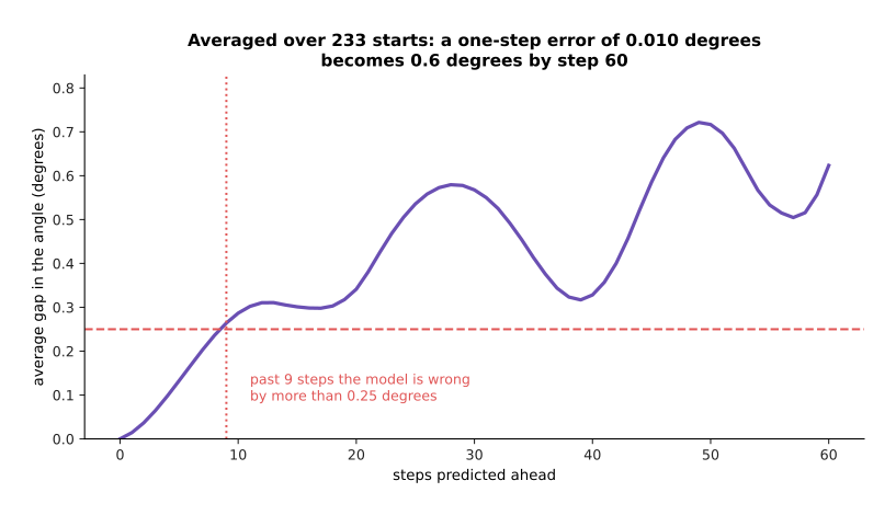
Over the 233 of 600 test runs that never touch the hard stop, the gap grows from 0.014 degrees one step ahead to 0.623 degrees sixty steps ahead. It passes a quarter of a degree at step 9, which is 0.45 seconds.
A one-step error of a hundredth of a degree has become six tenths of a degree in three seconds, which is forty-five times larger. The same run can be drawn as a path through angle and speed together, which is called a phase chart. On a phase chart the angle is across and the speed is up, so one point holds the whole state at one moment, and a swing back and forth becomes a loop.
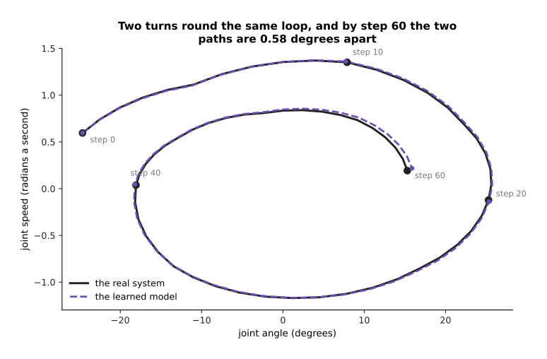
The two paths go twice round the same loop, and by step 60 they are 0.58 degrees apart.
The obvious reaction is to fit the model on more data, and the measurement says that this does not work. The next picture measures the same six fitted models in two ways: the left panel gives the error one step ahead, and the right panel gives the gap sixty steps ahead.
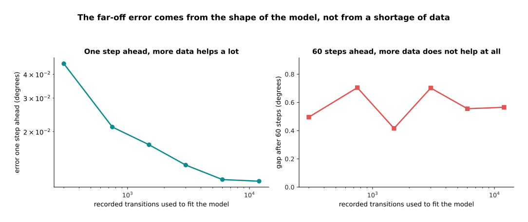
Going from 300 recorded transitions to 12,000 cuts the one-step error by four times over, from 0.0454 to 0.0110 degrees. Over the same range the sixty-step gap changes by a factor of only 1.69, and it changes in no particular direction.
The reason is in the last picture of section 1. The model's error is not noise that averages away with more examples. It is a small bias left over from the fact that a curve made of squares is not a sine, and a rollout adds that bias up step after step. No amount of data removes a bias in the shape of the model. So the rule people draw from this is to trust a learned model for a horizon measured in tenths of a second, and to find that limit by measuring it rather than by assuming it.
4. Planning against a learned model#
Now that there is a model, and a known limit on how far ahead it can be trusted, it can be used to choose what to do. Model-based planning means trying several action sequences inside the model, scoring what each one leads to, and then running the first action of whichever scored best. Nothing touches the robot while this happens, which is the appeal, because a bad idea costs a few milliseconds of arithmetic rather than a collision.
Scoring means giving each predicted step a number that says how bad it is, and adding those numbers up along the sequence. Lower is better, so the planner keeps the sequence with the smallest total. The next picture draws the score used here against the joint angle, with the arm standing still and no torque applied.
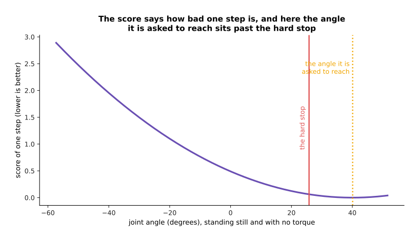
The score here is the squared distance from the angle the planner is told to reach, plus small penalties for moving fast and for using torque. The angle it is told to reach sits past the hard stop, which matters in section 6.
The simplest way to choose a sequence, and still a common one, is to draw the candidate sequences at random. The next picture shows one such decision.
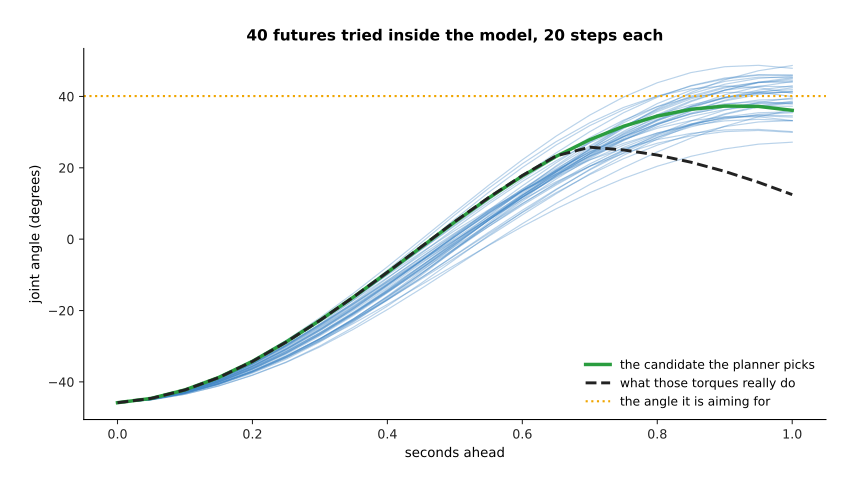
Forty random torque sequences of twenty steps each are run inside the model, which is 800 model steps for one decision. The one the planner picks ends at 36.11 degrees inside the model, while those same torques on the real arm end at 12.49 degrees.
That gap is section 3's growing error turning into a wrong decision, and section 6 comes back to it. First comes the arithmetic of how many futures can be tried at all, because it decides which kinds of world model are usable.
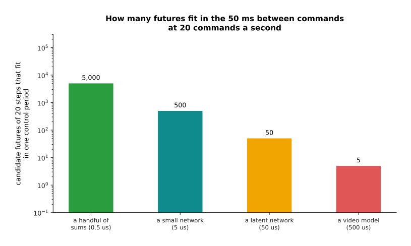
At 20 commands a second there are 50 milliseconds between commands. That holds 5,000 candidate futures of twenty steps if one model step costs half a microsecond, 500 if it costs 5 microseconds, 50 if it costs 50 microseconds, and 5 if it costs 500 microseconds.
The cost is always the number of candidates multiplied by the number of steps ahead, because every step of every candidate is one call of the model. The next picture draws that product.
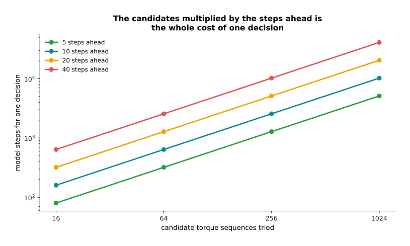
Doubling the candidates or doubling the steps ahead doubles the work in the same way.
A model small enough to run in a few microseconds leaves room to search properly. A model that takes half a millisecond a step leaves room for five guesses, which is not a search at all. That line of arithmetic is why latent dynamics models of a few dozen numbers are used for planning on robots, and video models are not. Within those limits, more candidates do give a better plan.
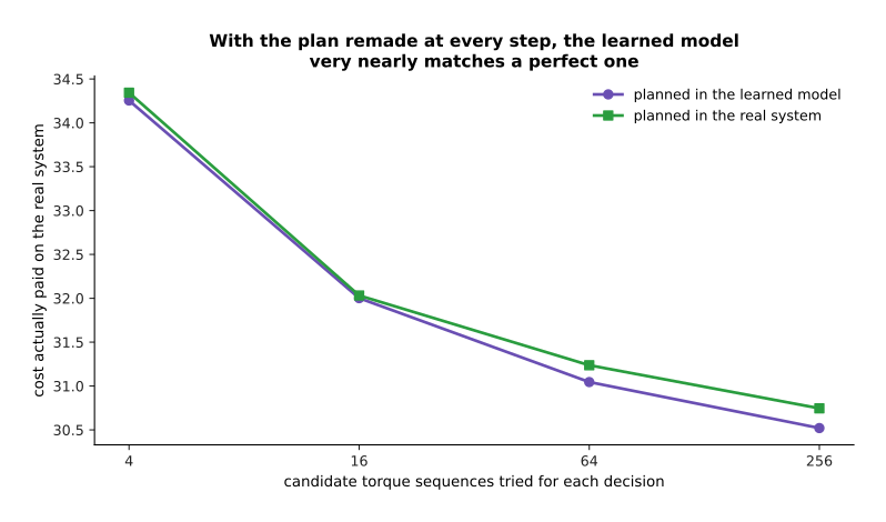
Going from 4 candidates to 256 cuts the cost actually paid from 34.3 to 30.5. Planning inside the learned model gives almost exactly the same result as planning inside the real system.
That last part looks like it contradicts section 3, and it does not. The plan is thrown away and made again from a fresh measurement at every step, so the model is only ever trusted for the length of one decision, and section 3 said the model is excellent over one step. The next picture shows how much work is discarded that way.
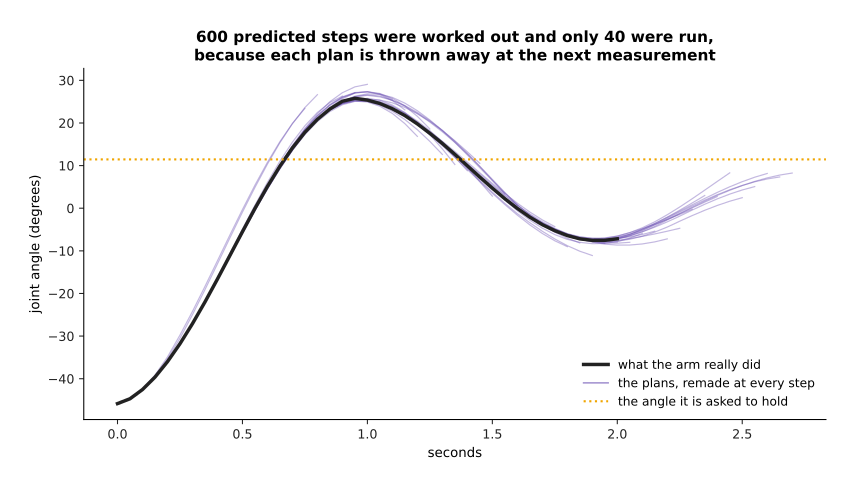
Forty decisions of fifteen steps each work out 600 predicted steps, and only 40 of them are ever run, which is 6.7 per cent.
Remaking the plan is what makes a drifting model usable, and the price of not doing it can be measured. The next picture runs the same planner while a steady extra pull acts on the arm that the model knows nothing about.
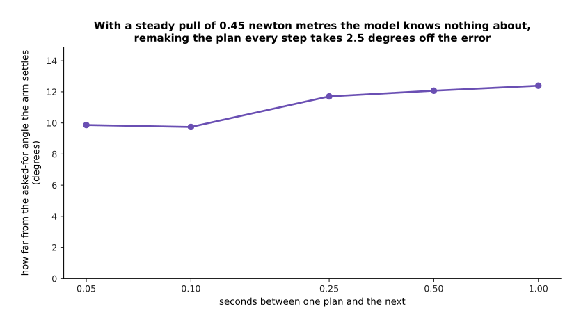
With a steady pull of 0.45 newton metres that the model knows nothing about, remaking the plan at every step leaves the arm 9.87 degrees from the angle it was asked to hold, while remaking it once a second leaves 12.39 degrees.
So planning against a learned model works, and it works because the plan is constantly discarded. Two things decide whether it is possible at all: the cost of one model step, and the horizon the model can be trusted over. Both get much worse when the model predicts pictures, which is the next section.
5. Video prediction and neural simulators#
The world models above all predict a short list of numbers that somebody had to design. The alternative that attracts the most attention skips that step and predicts the picture itself, using the generative machinery from diffusion. A video prediction model takes a few frames and an action, and generates the frames that come next. People want one because it can be trained on material that nobody had to label.
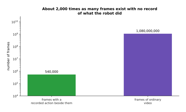
A full recording of 1,800 robot episodes is 540,000 frames, each with a recorded action beside it. Ten thousand hours of ordinary video at 30 frames a second is 1,080,000,000 frames, which is about 2,000 times as many.
That ratio is the whole argument, and it is a real one, because a video model can learn from all that video what objects do when they are pushed, dropped or poured. No amount of robot recording would show all of that. What such video cannot teach is which action caused which change, because nobody wrote the actions down. So a model trained on video still has to be trained on recorded episodes before it can be planned with, and the video stage is a good start rather than a replacement.
The second cost is time. The next picture measures the same comparison at two scales: the left panel counts the numbers written for one predicted step, and the right panel counts them for one whole planning decision.
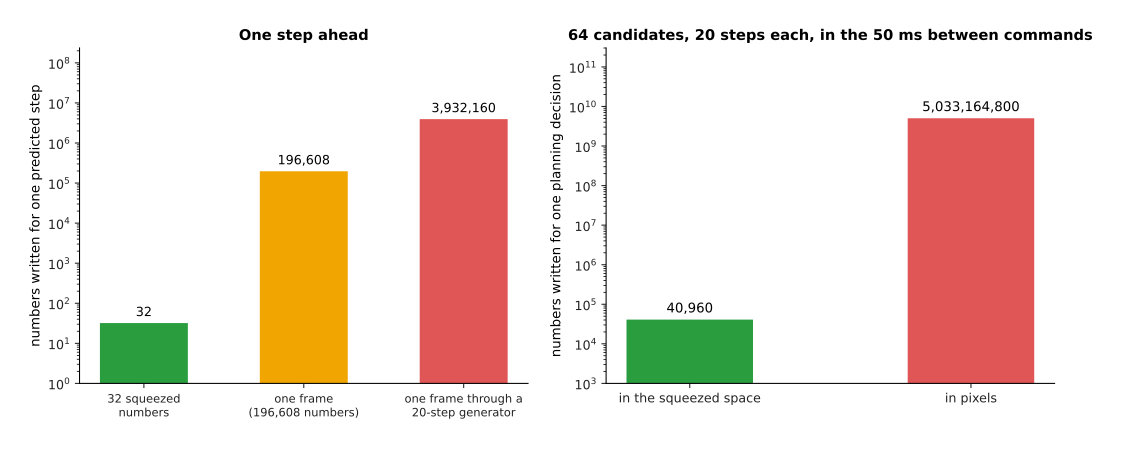
One predicted frame at 256 by 256 pixels in colour is 196,608 numbers. A generator takes several passes to produce one frame, and each pass removes a little of the noise, so it is called a denoising step. Twenty denoising steps write 3,932,160 numbers for one frame. One planning decision with 64 candidates twenty steps long therefore writes 5,033,164,800 numbers in pixels, against 40,960 numbers in a 32-number squeezed space, which is 122,880 times the work.
Put that beside section 4's budget of 50 milliseconds and it settles the question. Nobody plans at a robot's control rate by generating video. Video world models are used in three other ways instead. They pretrain the squeezed-down space that a fast latent model then predicts in. They are run slowly, a few times a second, to check whether a plan looks sensible while a fast policy does the moving. And they are run offline, to generate training material for a policy rather than to decide anything in the moment.
That last use is what people mean by a neural simulator: a learned model used in place of a hand-written physics engine, to produce the practice runs a policy learns from. The attraction is real. A hand-written simulator must be told the mass of every part, the friction of every surface and the shape of every object, and getting those numbers wrong is the main reason policies trained in simulation fail on the real robot. A learned simulator gets all of it from recordings instead. The limitation is that it only knows the parts of the world the recordings covered, and the next picture measures that. Both panels describe the same two sets of steps: the left one measures the error in the angle, and the right one measures it in the speed.
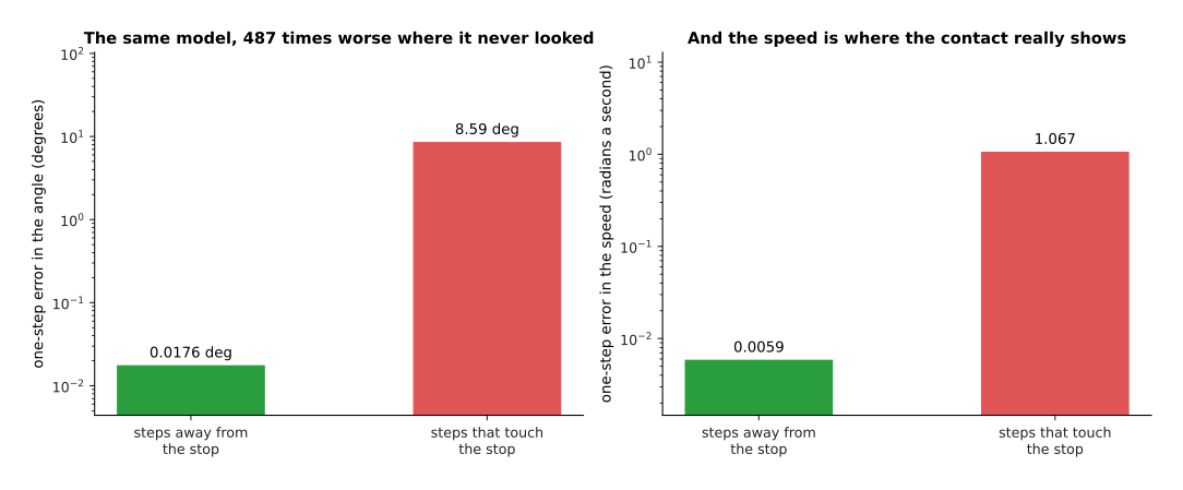
The same learned model is wrong by 0.0176 degrees for a step that does not touch the hard stop, and by 8.59 degrees for one that does, which is 487 times worse. In the speed it is 181 times worse.
So a neural simulator is not a cheaper physics engine. It is a different thing with a different failure. A hand-written engine is wrong everywhere by however much its numbers are wrong, and that error is roughly the same whatever the robot does. A learned one is nearly perfect where it was shown and arbitrarily wrong where it was not, and contact is almost always in the second group.
6. When the model gets the physics wrong#
The last section said that a learned model is arbitrarily wrong where it has not looked. This section shows what that looks like, because "it predicted the wrong physics" means something very specific once you watch it happen.
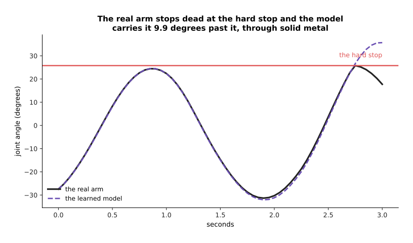
The real arm reaches the hard stop after 2.75 seconds and goes no further. The model carries it 9.9 degrees past the stop, up to 35.7 degrees.
The model is not confused and it is not uncertain. It gives a clean, confident answer in which the arm passes through solid metal, because nothing in the 11,522 transitions it was fitted on ever showed it that there was anything there. A model has no way of representing a thing it was never shown, and that is the most important sentence on this page, because contact is exactly what a robot arm spends its time doing and exactly what demonstrations avoid.
One run could be unlucky, so the next picture averages over 600 runs, split into the ones that reach the stop and the ones that do not.
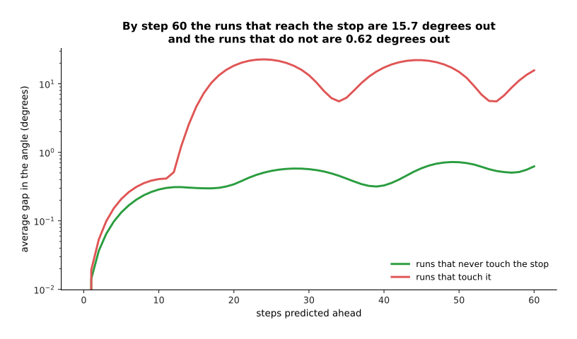
Averaged over the 367 runs that touch the stop, the gap reaches 15.7 degrees by step 60. Over the 233 runs that do not touch it, the gap reaches 0.62 degrees.
The wrongness is not confined to collisions, either, because even in open space the model quietly breaks a rule that the real world keeps, which is that energy is never created. The next picture measures the same run in two ways: the left panel gives the angle over time, and the right panel gives the energy the arm holds.
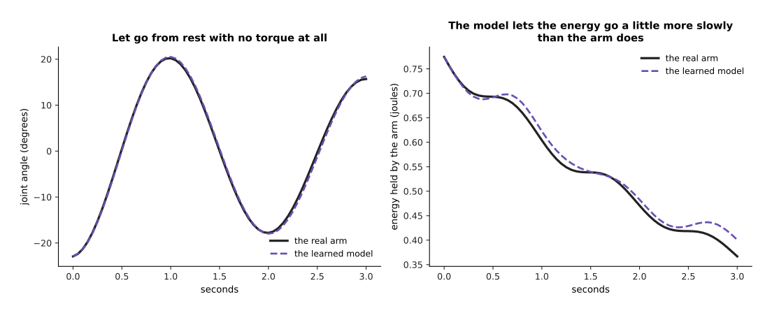
Let go from rest with no torque at all, the real arm swings up to 20.2 degrees, which stays clear of the stop. Its energy falls from 0.7744 to 0.3668 joules as friction takes the energy away. The model's version falls only to 0.4007 joules. The difference is 4.4 per cent of the starting energy, and nothing in the real system produced it.
Energy is not something the model was told about, so nothing stops it from making a little. Four per cent over three seconds sounds harmless, and on its own it is. However, a planner searching for the sequence that reaches a goal fastest is searching for exactly the sequences where this invented energy helps it. That is the last failure to show. The next picture measures the same six searches in two ways: the left panel gives the three costs, and the right panel gives the two gaps between them.
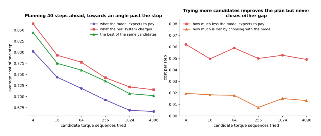
Planning forty steps ahead towards an angle that is past the hard stop, the model expects to pay 0.8020 a step with four candidates, and 0.6664 with 4,096. The real system charges 0.8641 and 0.7154 for the same plans. So the model expects to pay between 0.0490 and 0.0621 a step less than it really pays, however hard the planner searches.
Two things there deserve naming. The first is that the model always expects to do better than it does, and searching harder does not close that gap. The planner chooses the sequence the model scores best, and the model scores a sequence best partly when it is most wrong about it. The second is the gap between the red line and the green one. That is what the planner loses by choosing with the model instead of with the truth, and it stays between 0.0073 and 0.0195 a step however many candidates are tried. Trying more futures buys a better plan, and not a more honest one.
The list of what people do about all of this is short, and every item on it is hard. They keep the planning horizon inside the range the model was measured to be trustworthy over, which section 3 put at tenths of a second here. They remake the plan from a fresh measurement at every step. They add a penalty for plans that go where the recording was thin, so that the planner stops being rewarded for finding the places the model has not seen. And they go and record the situations the model is worst at, which for an arm means deliberately recording contact rather than only success.
7. Where to read next#
- Starting a model of your own is the next chapter, and it answers the question these twelve chapters leave open: you know how these models work, so how do you begin making one.
- Running and evaluating a model comes after that chapter, and it takes the latency and honesty arguments of sections 4 and 6 and applies them to testing a model properly on a real robot.
- Reinforcement learning explains the learning-by-trying side of this, and a world model is what lets that trying happen inside a model instead of on the robot.
- Diffusion explains the generative machinery that a video prediction model is built from, including why it takes many steps to produce one frame.
- The map of models is the closing page of this book, and it puts world models beside every other family in one place.
- World models in the next book is the catalogue for this family, and learned dynamics models, video prediction models and learned simulators give the named models of each kind and what each one costs.
8. Using it in Python#
Section 1 fitted a dynamics model with one least-squares solve, and section 3 rolled it forward until it drifted. Both are short enough to write out in full. The code below does what the pictures on this page do, on the same simulated joint, so you can change the numbers and watch the horizon move.
import numpy as np

G, L, M_ARM, DAMP, DT, STOP = 9.81, 1.0, 1.0, 0.25, 0.05, 0.45

def true_step(s, u):                       # section 1: the real system, with a hard stop
    th, om = s[..., 0], s[..., 1]
    om = om + DT * (-(G / L) * np.sin(th) - DAMP * om + u / (M_ARM * L ** 2))
    th = th + DT * om
    hit = th > STOP
    return np.stack([np.where(hit, STOP, th), np.where(hit, 0.0, om)], axis=-1)

def features(s, u):                        # section 1: ten simple combinations
    th, om = s[..., 0], s[..., 1]
    return np.stack([np.ones_like(th), th, om, u, th**2, om**2, u**2,
                     th*om, th*u, om*u], axis=-1)

rng = np.random.default_rng(2)             # collect a recording of the arm moving
s = np.stack([rng.uniform(-1.0, -0.15, 400), rng.uniform(-0.8, 0.8, 400)], axis=1)
rows, acts, nexts = [], [], []
for _ in range(30):
    u = rng.uniform(-1.1, 1.1, 400)
    s2 = true_step(s, u)
    rows.append(s); acts.append(u); nexts.append(s2); s = s2
X = features(np.concatenate(rows), np.concatenate(acts))
Y = np.concatenate(nexts) - np.concatenate(rows)
W = np.linalg.solve(X.T @ X + 1e-6 * np.eye(10), X.T @ Y)    # the whole fit

def learned_step(s, u):                    # section 3: the model, run on its own output
    return s + features(s, u) @ W

start, torques = np.array([-0.8, 0.0]), rng.uniform(-1.1, 1.1, 60)
a = b = start
for k, u in enumerate(torques):            # one rollout in each, same torques
    a, b = true_step(a, np.array(u)), learned_step(b, np.array(u))
    if k + 1 in (1, 10, 30, 60):
        print(f'after {k+1:2d} steps the gap is '
              f'{np.degrees(abs(a[0] - b[0])):.4f} degrees')
NumPy is doing one thing for you here: the least-squares solve on the line that makes W.
That line is the entire training of this world model. On a real robot it becomes a network
trained by gradient descent over camera pictures, with PyTorch handling the gradients, but
the loop does not change. Collect transitions, fit a one-step predictor, run it forward.
What no library decides is everything the pictures measured. You choose how many numbers to reduce a picture to, and section 2 showed that eight numbers can hold 90.86 per cent of a picture while reading the gripper no better than guessing. You choose how far ahead to plan, and section 3 put the limit here at about nine steps, which you have to measure for your own system rather than guess. You choose how often to remake the plan, and section 4 showed that remaking it at every step is what makes a drifting model usable at all.
One thing to notice is that the gaps this code prints are larger than section 3's. The snippet keeps every recorded transition, including the few that touch the hard stop, and the single rollout it runs reaches the stop once. So it is printing section 6's failure rather than section 3's steady drift. Add a line counting how many steps of the real path sit at the stop, and the two kinds of error separate.
The last line of the loop is the one to take away. Print the gap at a few horizons, on your own system, before you trust the model for anything. The one-step number will look excellent and tell you almost nothing, and the number at thirty steps decides whether planning against the model is going to work.