Models That Act — Vision-language-action models

The page before this one, diffusion and flow policies, showed how a generative model can write a whole piece of movement at once. It left one problem open. A diffusion policy or a flow policy is trained on demonstrations of one job, so it does that one job and nothing else. This page is about the kind of model that removes that limit. It takes a sentence as well as a picture, and the sentence says which job to do.

A vision-language-action model is one trained model that reads camera pictures and a written instruction, and gives back the numbers that move a robot arm. The name is a list of what goes in and what comes out. People usually shorten it to VLA. The point of the design is that one model covers many jobs, because the job is named in words instead of being built into the weights. The weights are the numbers inside the model that training sets.

This page is for a reader who has read the two pages before it. You should already know what a policy is in the robot sense, what behaviour cloning is, and what an action chunk is. All three are explained on behaviour cloning and action chunks. You should also have read vision-language models, because the main part of this model is a vision-language model, and that part is not explained again here.

The page answers four questions. What is this model made of? How is a movement written down, so that a model built to predict words can produce one? How is it trained, so that learning to move does not destroy what the model already knew? And what does it really carry over to situations it was never trained on? Every number in the pictures is worked out by docs/diagrams/models_that_act_2.py. The robot episodes in those pictures are simulated from smooth invented curves, but everything done to them is real arithmetic.

Contents#

What a vision-language-action model is
The body: a vision-language model with an action output
Way one: every action number becomes a token
Way two: a small continuous action head
Co-training: robot episodes and web pictures together
Cross-embodiment: episodes from many different robots
What generalisation really looks like, and what it costs to run
How the task is given: words, and then a video
Where to read next
Using it in Python

1. What a vision-language-action model is#

Start on the outside of the model. Once you can see what goes in and what comes out, everything inside is easier to follow. The picture below shows one call of the model. A call means one run of the model, from its input to its output. The sizes in the picture are worked out for two cameras of 224 pixels by 224 pixels and an arm with six joints.

Two camera pictures cut into 16 by 16 grids of patches, an instruction box and a joint
state box, all feeding one model, with a table of ten rows by seven columns of joint
movement numbers coming out of
it — Two camera pictures cut into 16 by 16 grids of patches, an instruction box and a joint state box, all feeding one model, with a table of ten rows by seven columns of joint movement numbers coming out of it

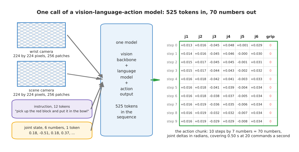
One call takes 525 tokens in and gives back 70 numbers, which are ten steps of seven numbers each.

A token is one item in the list of things the model reads. Each camera picture is cut into squares of 14 pixels by 14 pixels, and each square becomes one token. That gives 256 squares for one camera, so 512 for the two cameras together. The instruction is 12 tokens, because it has eleven words and one marker at the end. The six joint readings are packed into one more token. So the model reads 512 plus 12 plus 1, which is 525 tokens. What comes out is ten steps of six joint movements and one gripper command, which is 70 numbers. The arm takes 20 commands a second, so those ten steps cover half a second of movement.

This arrangement is worth building because the instruction changes the answer. The next picture keeps the same camera pictures and the same joint readings, and shows what two different instructions ask the arm to do.

Two line charts side by side, each with six coloured lines of commanded joint movement
over ten steps, and the two sets of lines have clearly different shapes under the two
instructions — Two line charts side by side, each with six coloured lines of commanded joint movement over ten steps, and the two sets of lines have clearly different shapes under the two instructions

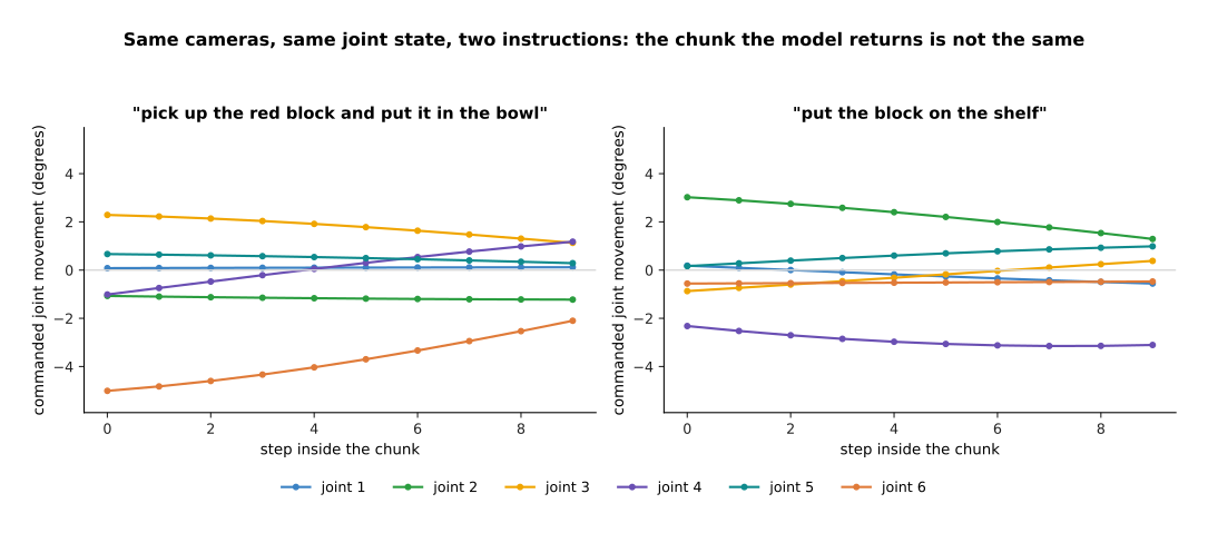
The two chunks differ by 2.53 degrees a joint a step. In an average step a joint moves 1.32 degrees, so the difference between the two answers is larger than the movement itself. This means the instruction decides the answer rather than adjusting it slightly.

A policy trained for one task cannot do this, because it has no input that says which task to do. The difference shows up in two places. The first is how much data one trained model learns from, which the next picture measures.

A bar chart comparing 150 episodes and 45,000 frames for one per-task policy with 1,800
episodes and 540,000 frames for one shared
policy — A bar chart comparing 150 episodes and 45,000 frames for one per-task policy with 1,800 episodes and 540,000 frames for one shared policy

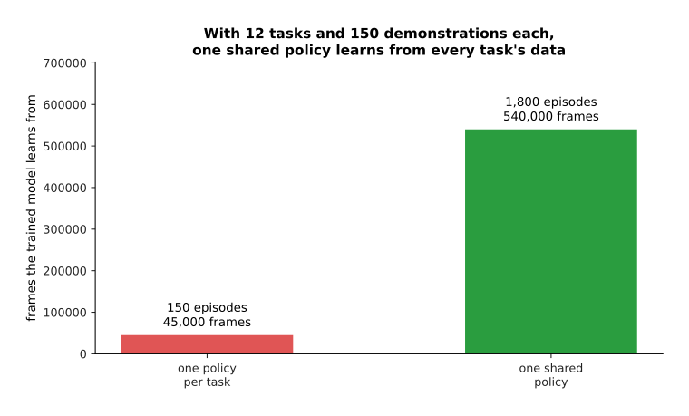
With twelve tasks and 150 demonstrations of each, a separate policy for one task learns from 150 episodes, while one instruction-reading policy learns from all 1,800.

That is 45,000 frames against 540,000 frames. The shared model also reuses what it learned about one task when it does another, because the same weights serve every task. The second place the difference shows up is how many trained models you have to keep working, and the next picture counts them.

A line chart where the number of separate models rises by one for each new task, while
the count for one shared policy stays at one all the way
across — A line chart where the number of separate models rises by one for each new task, while the count for one shared policy stays at one all the way across

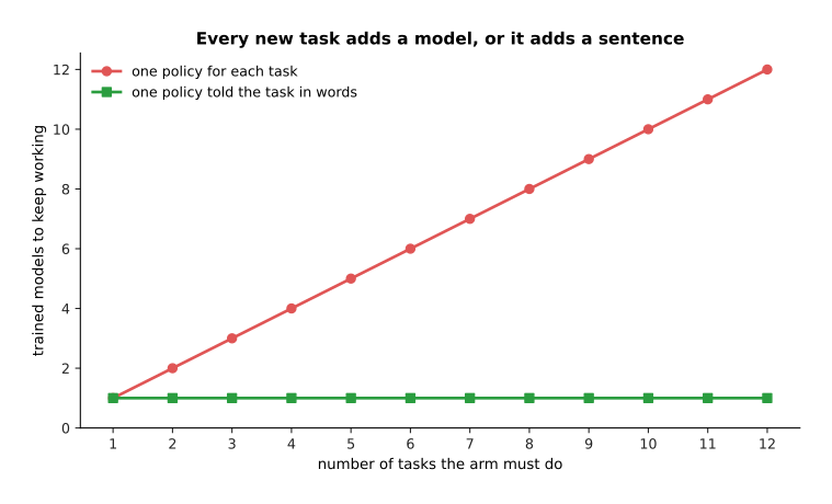
Every task you add brings another model to train, test and keep working, unless the task is given to one model in words.

The cost of the shared model is that it is much larger and much slower than a policy for one task. Section 7 measures that cost.

2. The body: a vision-language model with an action output#

The next question is what sits between the input and the output. The answer is a model you have already met. A vision-language-action model is a vision-language model with an action output added to it. The body of a model means its main part, which here is the part that looks at the pictures and reads the instruction. Almost all of the model was built to read pictures and write words, and only the last part is new.

The picture below lists the stages of one call. Read it from the top down: each row names a stage and gives the arithmetic for that stage.

Seven stacked rows, each naming one stage and giving its arithmetic, from two camera
pictures of 301,056 numbers at the top down to an action chunk of 70 numbers at the
bottom — Seven stacked rows, each naming one stage and giving its arithmetic, from two camera pictures of 301,056 numbers at the top down to an action chunk of 70 numbers at the bottom

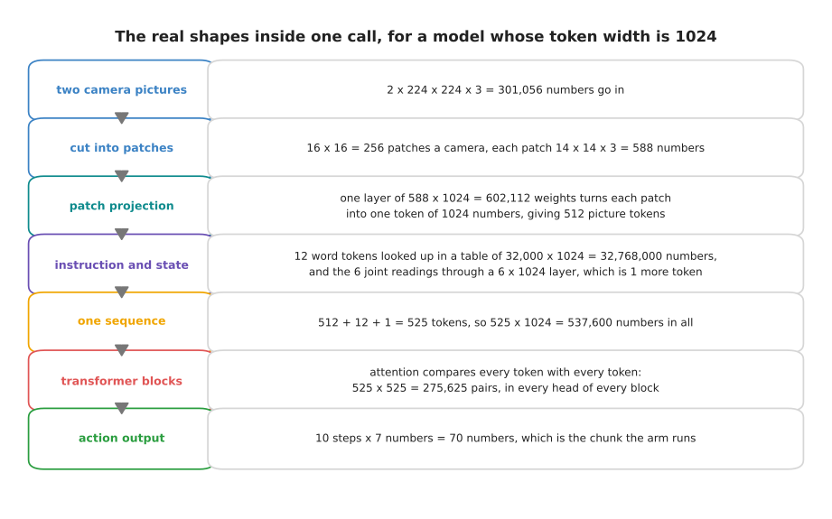
Every number here follows from three choices: the picture size, the patch size and the token width. The token width is how many numbers the model uses to hold one token.

Two colour pictures of 224 by 224 pixels are 301,056 numbers in total. Each patch is 588 numbers, because a patch is 14 by 14 pixels in three colours. One layer of 602,112 weights turns each patch into a token of 1,024 numbers. The words are looked up in a table of 32,000 rows by 1,024 columns, which holds 32,768,000 numbers. The 525 tokens together are 537,600 numbers. Inside every attention layer the model compares every token with every token, which is 275,625 pairs. Attention is the step where each token is allowed to look at the others, and this count of pairs is why the camera resolution is such an expensive choice.

The next picture shows what a sharper picture costs. The two bar charts measure the same four picture sizes in two ways: the left one counts tokens, and the right one counts the work attention does.

Two bar charts over the same four picture sizes, the left showing tokens rising from 525
to 4,621 as the picture grows from 224 to 672 pixels, the right showing the attention work
rising to 77.5 times the starting
cost — Two bar charts over the same four picture sizes, the left showing tokens rising from 525 to 4,621 as the picture grows from 224 to 672 pixels, the right showing the attention work rising to 77.5 times the starting cost

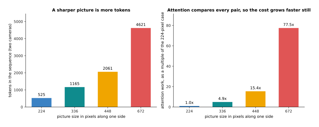
Going from 224 to 672 pixels a side multiplies the tokens by about nine, and it multiplies the attention work by 77.5.

The reason is that doubling the width of a picture puts four times as many patches in it. Attention compares every pair of tokens, so four times as many tokens is about sixteen times as much work. A robot that has to see a small screw pays that price at every call. This is why these models usually take one wide view of the scene and one close view from a camera on the wrist, rather than one very sharp view of everything.

The new part of the model is the output. Something has to turn the model's last token of 1,024 numbers into the 70 numbers of a chunk, and how that is done is the real design choice. There are two ways, and the picture below puts them side by side with the number of weights each one needs.

A branch diagram from the model's last token into two boxes, the left describing a
32,768,000-weight output layer that produces 70 tokens one after another, the right a
364,358-weight head that produces all 70 numbers at
once — A branch diagram from the model's last token into two boxes, the left describing a 32,768,000-weight output layer that produces 70 tokens one after another, the right a 364,358-weight head that produces all 70 numbers at once

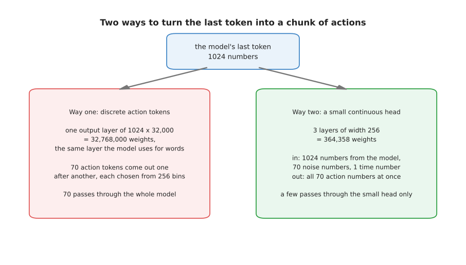
The first way reuses the model's own 32,768,000-weight word layer. The second way adds a small separate network of 364,358 weights, which is 90 times fewer weights.

The first way treats each action number as a word, by giving it a place in the vocabulary. The vocabulary is the fixed list of items a language model can choose from. The model then produces actions exactly as it produces text. The second way attaches a small network that produces the whole chunk directly. The next two sections take the two ways one at a time.

3. Way one: every action number becomes a token#

The first way starts from a mismatch of types. A language model chooses one entry from a fixed list, while a joint movement can take any value at all. Action tokenisation fixes that mismatch. It divides the range of each action number into bins, and treats each bin as one entry in the vocabulary. A bin is one small interval of values, and every value inside it is replaced by the value in the middle of that interval. Saying "bin 137" is then the same kind of act as saying the word "bowl". The range that the bins cover is decided from the training data rather than from the arm's data sheet.

The next picture shows what that looks like for one joint. The two panels show the same recorded movements at two scales: the left panel shows all of them, and the right panel shows a close-up of twelve bins near zero.

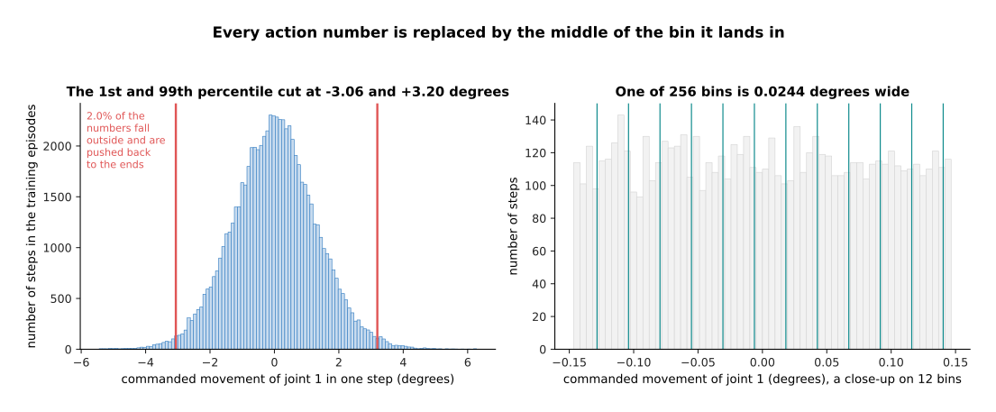
A histogram of one joint's commanded movement with two red lines marking the 1st and 99th percentile, beside a close-up of the same histogram crossed by twelve evenly spaced bin edges

For this joint the 1st and 99th percentile of the recorded movements fall at -3.06 and +3.20 degrees. A percentile is a cut point in the sorted data: 1 per cent of the recorded movements are below the 1st percentile, and 1 per cent are above the 99th. With 256 bins, one bin is 0.0244 degrees wide.

Any value outside that range is replaced by the nearest end bin, which is called clipping. Clipping happens to 2.0 per cent of this joint's numbers. The only question left seems to be how many bins to use, and the measurement says that this stops mattering very quickly.

The next picture measures the error that binning causes, for six choices of how many bins to use. The left panel gives the error in degrees at the joint, and the right panel gives the same error in millimetres at the fingertip.

Two charts over the same six bin counts, the left showing the rounding error falling
steadily while the total error flattens out, the right showing the rounding error at the
fingertip falling from 0.587 mm at 32 bins to 0.018 mm at 1,024
bins — Two charts over the same six bin counts, the left showing the rounding error falling steadily while the total error flattens out, the right showing the rounding error at the fingertip falling from 0.587 mm at 32 bins to 0.018 mm at 1,024 bins

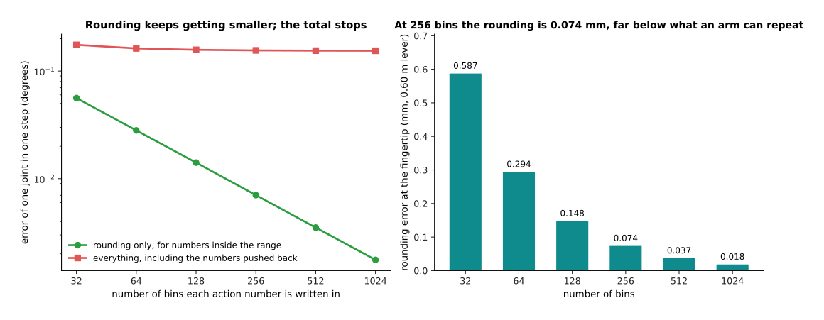
At 256 bins the rounding on its own is 0.0070 degrees a joint a step. That is 0.074 millimetres at a fingertip 0.60 metres from the joint, and the worst single rounding is 0.0125 degrees.

That is far below what any arm can repeat, so rounding is not what this method costs you. The cost is in the 2.7 per cent of numbers that fall outside the range and get clipped. Those are the fastest movements, and clipping always makes a movement shorter than it was. The model produces movements rather than positions, so each shortened movement is added to the ones before it, and the shortfalls add up.

The next picture shows four choices of range, all with the same 256 bins. The left panel gives the error of one step, and the right panel gives how far the fingertip has drifted after ten steps and after three hundred.

Two bar charts over the same four choices of range, the left showing the one-step error
at 256 bins, the right showing the fingertip drift after ten steps and after three hundred
steps — Two bar charts over the same four choices of range, the left showing the one-step error at 256 bins, the right showing the fingertip drift after ten steps and after three hundred steps

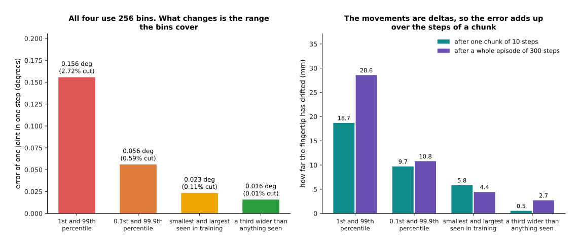
All four use 256 bins and differ only in the range the bins cover. That choice moves the one-step error from 0.156 to 0.016 degrees, and it moves the drift after one chunk from 18.70 to 0.54 millimetres.

Cutting the range at the 1st and 99th percentile clips 2.72 per cent of the numbers, and it leaves the fingertip 18.70 millimetres out of place after only ten steps. Cutting at the 0.1st and 99.9th percentile clips 0.59 per cent and halves that drift to 9.71 millimetres. Making the range a third wider than anything ever recorded leaves 0.54 millimetres, which is the floor set by rounding alone. So the number of bins is the part people argue about, and the range is the part that costs them millimetres.

The real price of this method is not accuracy but the number of tokens, because the model produces each action token in a separate pass. The next picture counts the tokens for three cases.

A bar chart of action tokens for three cases: 60 tokens for a ten-step chunk, 300 for a
fifty-step chunk, and 36 for the same fifty-step chunk kept as six frequency
terms — A bar chart of action tokens for three cases: 60 tokens for a ten-step chunk, 300 for a fifty-step chunk, and 36 for the same fifty-step chunk kept as six frequency terms

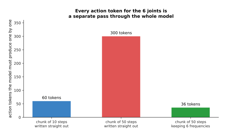
A ten-step chunk costs 60 tokens for six joints, and a fifty-step chunk costs 300. Describing the longer chunk by its first six frequency terms costs 36 tokens instead.

That last case needs explaining. It uses a discrete cosine transform, which rewrites a sequence of numbers exactly as a sum of waves of different speeds. Each wave in the sum is one frequency term. A demonstrated movement is smooth, so almost all of it is carried by the slowest few waves, and the fast waves can be dropped with little loss. The next picture measures how much is lost.

A curve of the error of a rebuilt fifty-step chunk against the number of tokens used,
falling steeply from 12 tokens to about 50 tokens and then flattening
out — A curve of the error of a rebuilt fifty-step chunk against the number of tokens used, falling steeply from 12 tokens to about 50 tokens and then flattening out

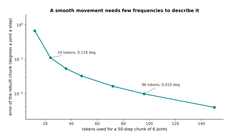
Keeping six terms a joint rebuilds the chunk to within 0.053 degrees using 36 tokens, and keeping four terms a joint rebuilds it to 0.110 degrees using 24 tokens, in place of 300.

Several real systems compress a chunk this way before turning it into tokens. That is the honest answer to the token count, rather than using fewer bins.

So action tokenisation is the simplest thing that can be done. It needs no new machinery, it trains with the loss the language model already used, and because actions live in the same vocabulary as words, the model can take robot data and text in the same batch. Its cost is one pass through the whole model for every number it produces.

4. Way two: a small continuous action head#

The second way keeps the same body and replaces the output. Instead of naming a bin, a small extra network called an action head takes the model's last token and produces all 70 numbers at once. The head is almost always generative, which means that it draws one of the answers that fit the situation instead of always giving the same one. In practice that means it is built with flow matching or with diffusion. The reason is given on diffusion and flow policies. A plain network trained with squared error, which scores an answer by the square of its distance from the demonstrated one, answers an ambiguous situation by averaging the possible movements, and the average of two good movements is usually a bad one.

A flow-matching head starts from a list of random numbers and walks it into a list of action numbers. The walk takes a few equal steps, and at each step the head predicts the direction to move in. The head in the pictures below is a real one. It is a small network of 59,750 weights, trained in NumPy on the simulated chunks by the method described on flow matching and other generators. It is smaller than the head counted in section 2, because what it is told about the situation here is the ten actions just before the chunk, rather than a token of 1,024 numbers from a vision-language model.

The first picture follows one list of random numbers through that walk, for four different numbers of steps.

A chart with four lines showing one list of random numbers walked into an action in one,
two, four and thirty-two steps, with the four lines ending at different
values — A chart with four lines showing one list of random numbers walked into an action in one, two, four and thirty-two steps, with the four lines ending at different values

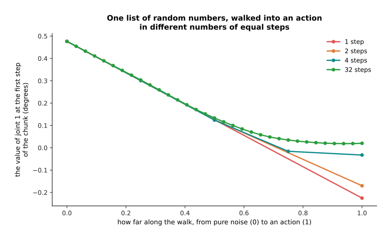
One big step lands this joint 0.245 degrees from where thirty-two small steps land it. Two steps land 0.190 degrees away, and four steps land 0.053 degrees away.

The paths are nearly straight, which is what flow matching is for, and that is why only a few steps are enough. The second picture starts twenty-four different lists of random numbers from the same situation and walks each of them.

Twenty-four pale lines starting far apart at the left of the chart and converging into a
narrow band at the
right — Twenty-four pale lines starting far apart at the left of the chart and converging into a narrow band at the right

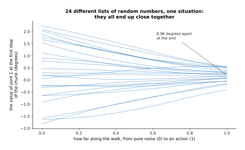
The twenty-four walks start 4.05 degrees apart and end 0.96 degrees apart. This means the head gives roughly the same answer whatever random numbers it starts from.

The number of steps trades exactness for time, and that trade can be measured. The next picture measures it against a very fine walk of 128 steps, which stands in for the exact answer.

A chart on logarithmic axes showing the distance from the 128-step answer falling from
0.615 degrees at one step to 0.007 degrees at thirty-two
steps — A chart on logarithmic axes showing the distance from the 128-step answer falling from 0.615 degrees at one step to 0.007 degrees at thirty-two steps

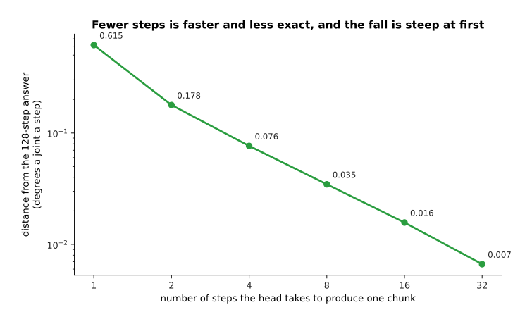
One step leaves the chunk 0.615 degrees out. Two steps leave 0.178, four leave 0.077, and eight leave 0.035 degrees, which is 0.363 millimetres at the fingertip.

Eight steps is already below what the arm can repeat. That is the argument for this design, because eight passes through a small head cost far less than seventy passes through the whole model. The next picture puts numbers on that. Both panels describe the same set of choices: the left one gives the time for one chunk, and the right one turns that time into how often the model can look at a fresh picture.

Two charts, the left a bar chart of the time to make one chunk, with action tokens at 310
ms against the head at about 33 ms, the right showing how many fresh looks a second each
choice allows — Two charts, the left a bar chart of the time to make one chunk, with action tokens at 310 ms against the head at about 33 ms, the right showing how many fresh looks a second each choice allows

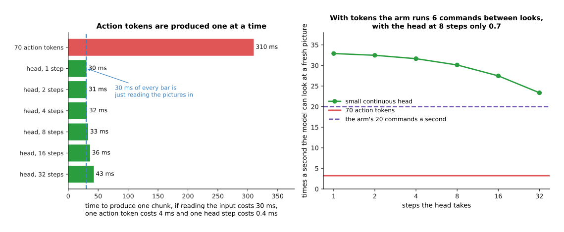
Suppose reading the 525 input tokens costs 30 milliseconds, one action token costs 4 milliseconds and one head step costs 0.4 milliseconds. Then 70 action tokens take 310 milliseconds, and the head at eight steps takes 33.2 milliseconds.

Those times decide how often the model looks at a fresh picture. With action tokens it looks 3.2 times a second, and with the head it looks 30.1 times a second. The arm takes 20 commands a second, so in the first case it runs 6.2 commands on information that is already out of date, and in the second case only 0.7 commands. A robot that has to react to a moving object is affected far more by that delay than by a hundredth of a degree of accuracy.

The last picture of this section compares the two outputs on one demonstrated chunk.

A line chart of one joint's movement falling over ten steps, with the demonstrated chunk
and the binned version lying on top of each other, and the head's two outputs following
them with a small
wobble — A line chart of one joint's movement falling over ten steps, with the demonstrated chunk and the binned version lying on top of each other, and the head's two outputs following them with a small wobble

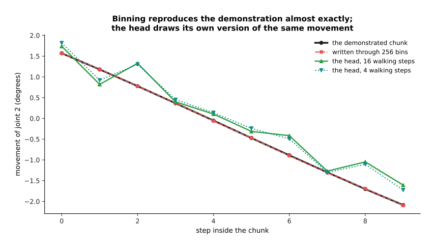
Binning moves this chunk by 0.0073 degrees, while the head's own chunk sits 0.326 degrees away from the demonstrated one. Over 200 situations the head lands 0.315 degrees a joint a step away from what was demonstrated.

The binned version copies a given chunk more exactly. That is true, and it is not the point. The head is not trying to copy one chunk. It is trying to draw one of the movements that fit the situation, and its wobble is partly the price of choosing between them. Part of the wobble is also the price of a small head trained for a few seconds in NumPy. So tokens are simpler and copy more exactly, while the head is roughly ten times faster and handles ambiguity properly. Most recent systems use the head.

5. Co-training: robot episodes and web pictures together#

Both ways of producing an action leave the same question open: how do you train the model without ruining it? The body knows what a bowl is because it was trained on an enormous number of ordinary pictures and texts. Training it on robot episodes alone destroys exactly that knowledge, for the reason set out under catastrophic forgetting on fine-tuning and adapters.

The effect is easy to measure on a small example. The next picture trains one small network on a general job, and then teaches it a second, robot-like job. Both panels show the same two measurements over the same training run. What changes between the panels is the data that the training uses.

Two charts of accuracy against training steps, the left showing the general job falling
from 96 to 59 per cent while the robot job rises, the right showing both staying high when
a quarter of the batches are general
data — Two charts of accuracy against training steps, the left showing the general job falling from 96 to 59 per cent while the robot job rises, the right showing both staying high when a quarter of the batches are general data

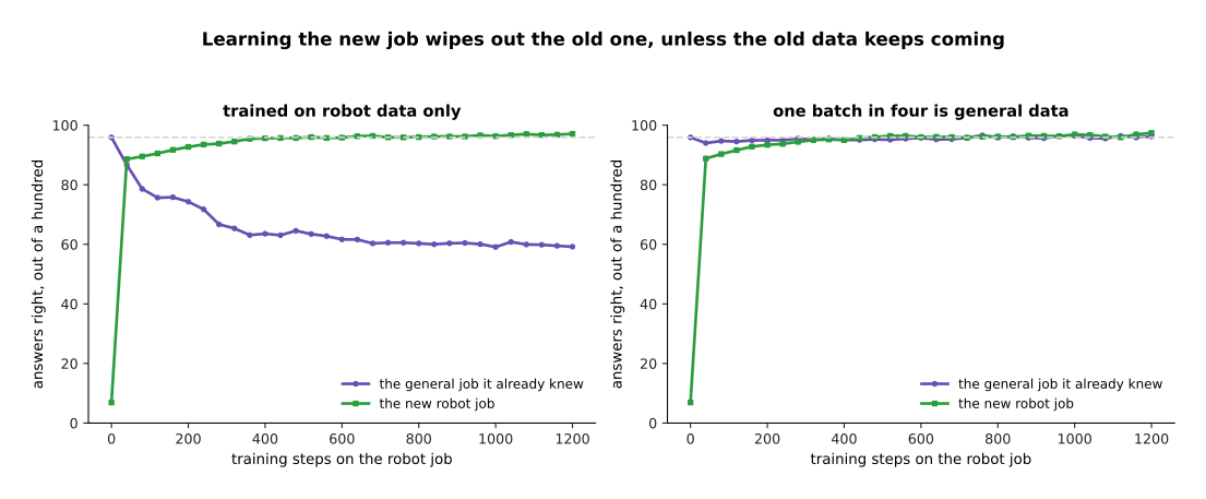
When only robot data is used, the general job falls from 95.9 per cent right to 59.2 per cent. When one batch in four is drawn from the general data, the general job stays at 96.2 per cent and the robot job still reaches 97.4 per cent.

Co-training is the name for the fix shown on the right. It means keeping the old data coming while the new job is learned, so that every batch is partly robot episodes and partly ordinary pictures and text. It is not a clever method. It is a refusal to stop showing the model the thing you want it to remember. The question that remains is how much of the old data is needed, and the next picture answers it.

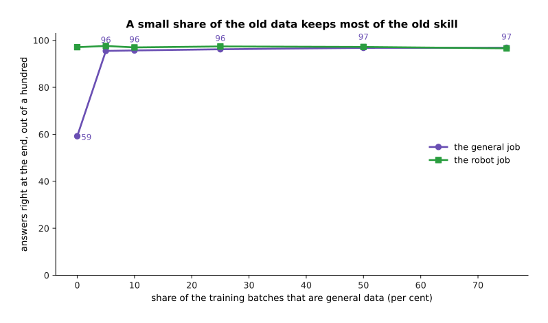
A line chart of the final accuracy on both jobs against the share of general data in the batches, where the general job jumps from 59 to 96 per cent as soon as five per cent of the batches are general

Five per cent of the batches brings the general job back from 59.2 to 95.5 per cent. Going all the way to three quarters gains only another 1.4 points, and by then the robot job has started to get slightly worse.

This has to be stated clearly, because the natural sizes of the two sets are nothing like the sizes you want. The next picture compares the two sets.

A bar chart on a logarithmic scale comparing 540,000 robot frames with 400,000,000
picture-and-text pairs from the
web — A bar chart on a logarithmic scale comparing 540,000 robot frames with 400,000,000 picture-and-text pairs from the web

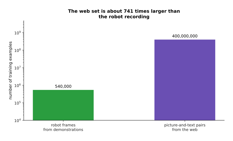
A recording of 1,800 episodes is 540,000 frames, while a modest web set is 400,000,000 picture-and-text pairs, which is about 741 times more.

If you simply mixed the two sets in those sizes, the robot frames would be a very small part of every batch. The next picture gives that share, beside the two shares a real training run would use.

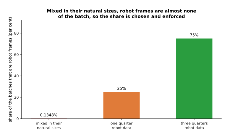
A bar chart of the share of the batches that are robot frames: 0.1348 per cent if the sets are mixed in their natural sizes, against the 25 per cent and 75 per cent a real run would choose

Mixed in their natural sizes, robot frames would be 0.1348 per cent of the batches.

At that share the model would barely learn to move. So the mixture is chosen on purpose and enforced by the sampler, which is the part of the training code that decides what goes into each batch. At three quarters robot data, every robot frame is seen about 2,222 times for each pass through the web set. The cost is that training takes longer, and that repeating the robot data that many times risks memorising it rather than learning from it.

6. Cross-embodiment: episodes from many different robots#

Co-training keeps old knowledge while robot data is added. The next question is where more robot data comes from. Cross-embodiment training pools episodes recorded on many different robots into one training set. Embodiment means the particular body the episodes were recorded on. The difficulty is that two robots do not use the same numbers for the same movement, even when they are doing the same thing.

The next picture shows one two-link arm in each panel. The two panels are the same job seen on two different bodies: each arm has to move its fingertip by the same small amount.

Two drawings of a two-link arm held at a fixed pose, each marked with the small joint
turns needed to move the fingertip twenty millimetres across and ten millimetres
up — Two drawings of a two-link arm held at a fixed pose, each marked with the small joint turns needed to move the fingertip twenty millimetres across and ten millimetres up

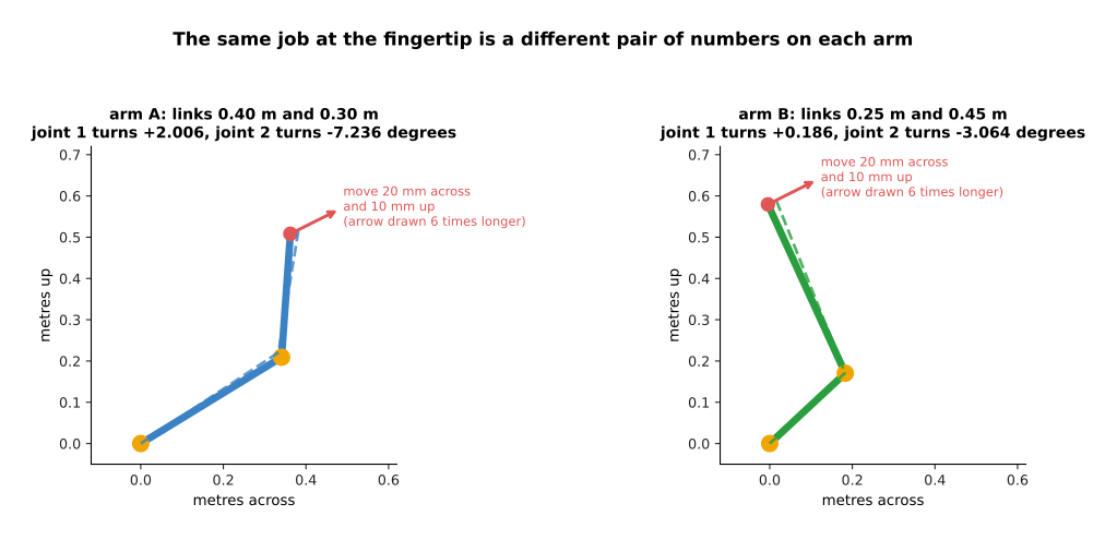
To move the fingertip 20 millimetres across and 10 millimetres up, an arm with links of 0.40 and 0.30 metres turns its joints by +2.006 and -7.236 degrees. An arm with links of 0.25 and 0.45 metres turns its joints by +0.186 and -3.064 degrees.

The same job at the fingertip is a different pair of numbers at the joints, so an action recorded on one arm means nothing on the other. There are two standard ways around this. The first describes the action at the fingertip: it records how far the gripper should move, and leaves each robot's own controller to work out the joint turns. The second scales each robot's numbers by that robot's own range, so that every robot's numbers fill the same interval.

The next picture shows the second way. The two panels are the same two recordings, drawn before and after the scaling.

Two histograms, the left showing arm A spread between about minus three and plus three
degrees a step while arm B sits in a narrow peak, the right showing both filling the same
range after
scaling — Two histograms, the left showing arm A spread between about minus three and plus three degrees a step while arm B sits in a narrow peak, the right showing both filling the same range after scaling

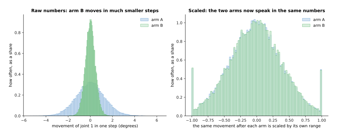
Arm A's first joint runs from -3.06 to +3.20 degrees a step, and arm B's runs from -1.07 to +1.11 degrees a step. After each one is divided by its own range, the two histograms lie on top of each other.

Now that the numbers are comparable, the two sets of episodes can be pooled. The result depends entirely on one detail, which the next picture measures.

A bar chart of three cases: arm B's own fifty episodes at 6.17 degrees of error, the
pooled set with a robot tag at 5.17 degrees, and the pooled set with no tag at 37.87
degrees — A bar chart of three cases: arm B's own fifty episodes at 6.17 degrees of error, the pooled set with a robot tag at 5.17 degrees, and the pooled set with no tag at 37.87 degrees

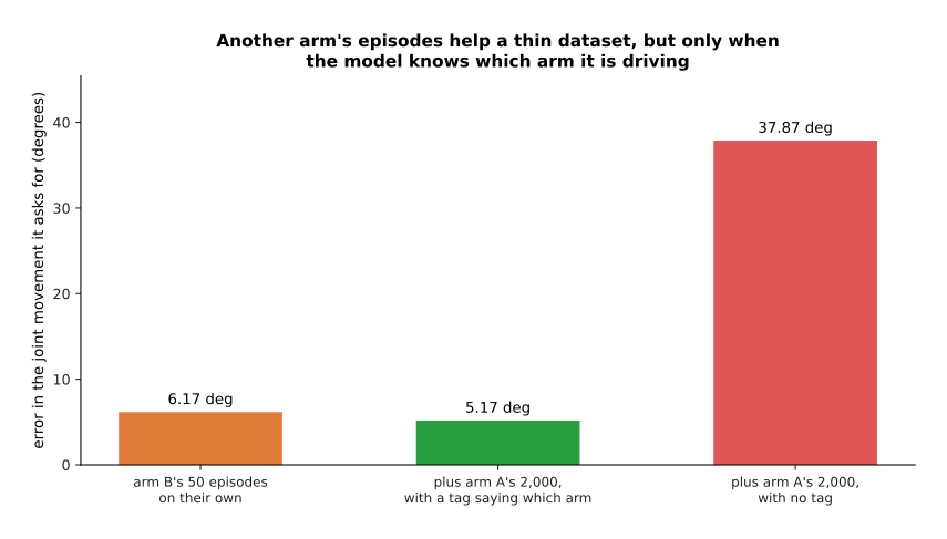
Adding 2,000 episodes from another arm cuts the error from 6.17 to 5.17 degrees when the model is told which arm it is driving. The same episodes raise the error to 37.87 degrees when the model is not told.

That third bar is why real systems add an embodiment tag to the input. A tag is an extra input that names the robot. A model that cannot tell the arms apart has to give one answer for both, and the average of two different answers fits neither. With the tag in place the pooled data helps, and the next picture says when it helps.

A line chart of error against the number of arm B examples, where the line for the pooled
data sits below the line for arm B's own data at twenty-five and fifty examples, and above
it from a hundred examples
onwards — A line chart of error against the number of arm B examples, where the line for the pooled data sits below the line for arm B's own data at twenty-five and fifty examples, and above it from a hundred examples onwards

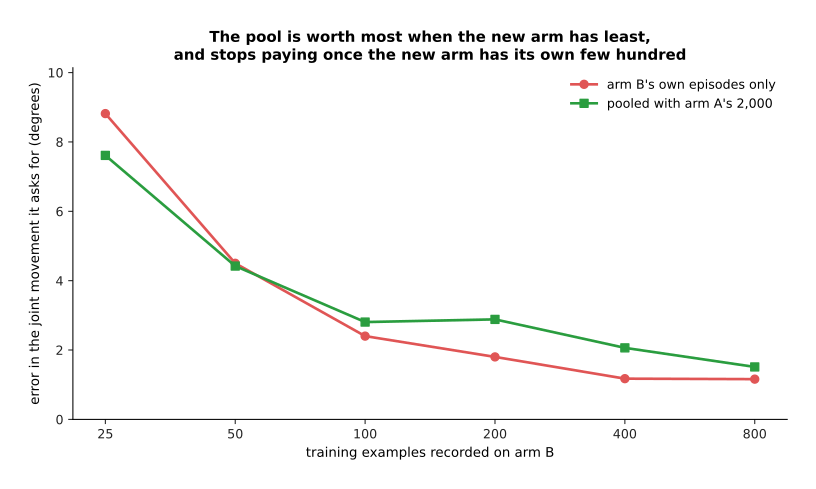
With 25 examples of its own, arm B does better with the pool, at 7.61 degrees against 8.82. With 50 examples the two are level. From 100 examples upwards, arm B's own data alone is the better teacher.

That is the honest shape of this result. Pooling helps most where a new robot has almost no data of its own, because the shared part of the job is learned from everybody's data at once. The shared part here is working out where the object is from the camera. Once the new robot has a few hundred episodes, the shared network has to split its capacity between bodies, and that costs more than the pooling gains. So cross-embodiment data gets a new robot started quickly, rather than making a well-supplied robot better.

7. What generalisation really looks like, and what it costs to run#

Pooling other robots' episodes was the last of the ways of getting more out of the data. This section is about what you get in return, which is the part most often described too generously. The useful question is not whether these models generalise, but which change they survive. The four changes below behave very differently.

The first change is moving the object, and that works inside limits that are easy to measure. The next picture shows where the training objects sat in the camera view.

A scatter of training object positions filling a square in the middle of the camera view,
with the whole view drawn as a larger dashed
square — A scatter of training object positions filling a square in the middle of the camera view, with the whole view drawn as a larger dashed square

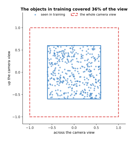
The objects used in training covered 36 per cent of the camera view, all of it in the middle.

The next picture measures the error at five distances from the middle of the view.

A bar chart of error by distance from the middle of the view, flat at 0.36 to 0.47
degrees for the three bands inside the trained area and rising to 2.62 and then 13.07
degrees for the two bands outside
it — A bar chart of error by distance from the middle of the view, flat at 0.36 to 0.47 degrees for the three bands inside the trained area and rising to 2.62 and then 13.07 degrees for the two bands outside it

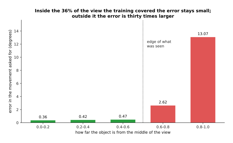
Inside the area the training covered, the error stays between 0.36 and 0.47 degrees. Outside it, the error rises to 2.62 degrees and then to 13.07 degrees.

So "the same task with the object moved" is really two claims. Moved inside the patch of table the demonstrations covered, the model is fine, and that is what people see in a demonstration video. Moved to a corner where nobody ever put an object, it is thirty times worse.

The second change is a new object. A new object of a kind the model has seen is a different case from a kind it has never seen, and the two separate cleanly. The next picture shows where the two kinds of object sit when an object is described by its width and its height.

A scatter of object widths and heights showing two clusters that do not overlap, tall
narrow objects in the upper left and wide flat objects in the lower
right — A scatter of object widths and heights showing two clusters that do not overlap, tall narrow objects in the upper left and wide flat objects in the lower right

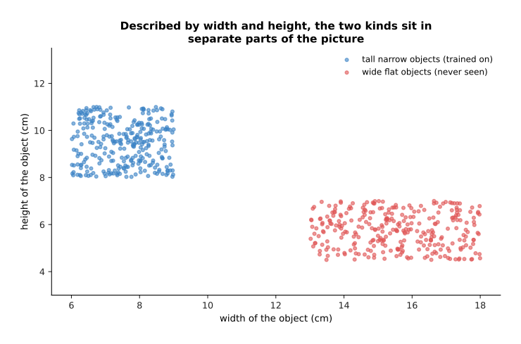
The objects used in training were tall and narrow. The wide flat objects sit in a part of this picture that the training never visited.

The next picture measures the error of the same learned rule on both kinds.

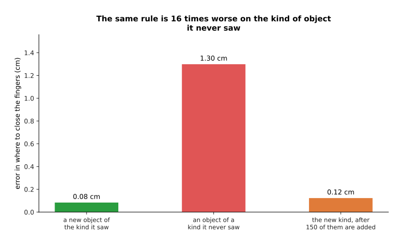
A bar chart of the error in where to close the fingers: 0.08 cm for a new object of the trained kind, 1.30 cm for an object of the untrained kind, and 0.12 cm once 150 of the new kind are added to training

A rule learned from 200 tall narrow objects places the fingers on a new tall narrow one to within 0.08 centimetres. It places them on a wide flat one to 1.30 centimetres, which is sixteen times worse. Adding 150 wide flat objects to the training brings that down to 0.12 centimetres.

The rule did not change between the two kinds, because in this simulation it is literally the same rule. The new kind sits in a part of the object's description that the training set never visited, so the model is guessing there rather than remembering. This means a model can fail on a new object even when the right answer follows from what it already knows.

The third change is rewording the instruction, and that one genuinely works. The next picture counts how many of the words in a new sentence already appeared in the training instructions.

A horizontal bar chart showing three rewordings of a trained task reusing 75 to 86 per
cent of the training vocabulary, while two new tasks reuse only 40 and 50 per
cent — A horizontal bar chart showing three rewordings of a trained task reusing 75 to 86 per cent of the training vocabulary, while two new tasks reuse only 40 and 50 per cent

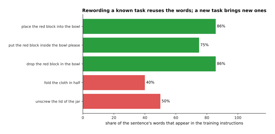
Three ways of saying the same trained task reuse between 75 and 86 per cent of the words used in training, while two new tasks reuse only 40 and 50 per cent.

Counting words is a crude substitute for measuring what the model does, so treat this picture as a hint rather than a result. Rewording really works for a different reason: the language half of the model was trained on far more text than the robot data holds, so it already treats those sentences as near neighbours. This is where the web pretraining helps directly.

The fourth change is a genuinely new task, and today that does not work. A model shown twelve tasks does not do a thirteenth one simply because you ask for it. People often call a success of that kind zero-shot, where zero-shot means working on something with no training examples of it at all. What is called zero-shot success here is almost always one of the first three cases instead.

The table below gathers the four changes, with a fifth row that separates the two cases of moving an object. Read it one row at a time: the first column names the change, the second says whether it works, and the third gives the measurement from this page that supports the verdict.

The change	Does it work?	What this page measured
The same task, object moved inside the area seen before	Works	The error stays near 0.42 degrees everywhere inside the area the training objects covered
The same task, said in different words	Usually works	75 to 86 per cent of the words in the reworded sentences already appear in the training instructions
The same task, object moved outside the area seen before	Does not work	The error grows to 13.07 degrees at the edge of the camera view
A new object of a kind the model never saw	Does not work	The error on the unseen kind is 16 times the error on a new object of a seen kind
A task the model was never shown	Does not work	Nothing in the training data says what the new words mean for the arm

That leaves the cost of running one of these models. A model that takes 310 milliseconds to produce a chunk cannot answer every 50 milliseconds, which is what an arm taking 20 commands a second would need. There are three things people do about it. The next picture is about the first two.

A chart on logarithmic axes of the shortest workable chunk length against the arm's
command rate, with three lines for three model speeds and a dashed line marking the
ten-step chunk used on this
page — A chart on logarithmic axes of the shortest workable chunk length against the arm's command rate, with three lines for three model speeds and a dashed line marking the ten-step chunk used on this page

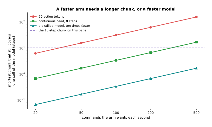
At 100 commands a second, the chunk has to cover at least 31 steps with action tokens, 3.3 steps with the head, and 0.3 steps with a distilled model ten times faster.

The first fix is a longer chunk, and it costs reaction time, because the arm keeps acting on a picture that is by then old. The second fix is a smaller model trained to copy the big one. That is the distillation described on making a model smaller and faster, and it costs some of the big model's knowledge. The third fix runs two models at two speeds: the big model runs slowly and decides what to aim for, and a small fast policy underneath moves the joints towards that aim. The next picture counts the steps of the fast policy that fit inside one call of the big one.

One long box standing for a single 310 millisecond call of the big model, with thirty-one
small boxes underneath it standing for the steps of a policy running 100 times a
second — One long box standing for a single 310 millisecond call of the big model, with thirty-one small boxes underneath it standing for the steps of a policy running 100 times a second

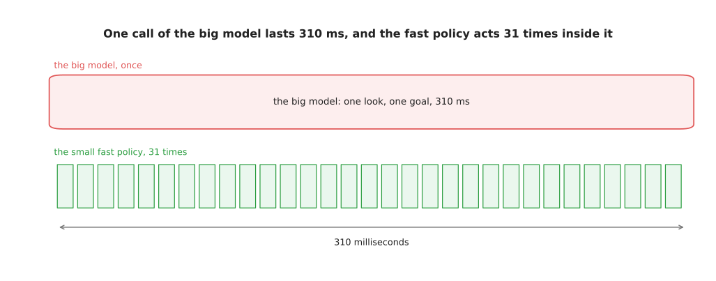
While the big model produces one chunk, a policy running at 100 commands a second takes 31 steps.

That split between a slow model and a fast one is now usual, and it leads into the next page, because a model that decides what to aim for is close to a model that predicts what will happen.

8. How the task is given: words, and then a video#

Everything above is about how a model turns pictures into movement. This section is about the other input, which is how the model is told which movement to make. In 2026 that is where the arrangement changed.

Every model described so far is told in words. The instruction "put the cup on the saucer" is turned into tokens, those tokens join the picture tokens, and attention mixes the two. Words are convenient, but a short sentence carries very little information. "Fold the towel" does not say which fold, in which order, or to what standard. The model therefore supplies the missing detail from the average of its training data rather than from what you wanted.

The alternative is to give the model an example of the task instead of a description of it. The example is a short video. It enters the model as more tokens, exactly as the instruction did, and attention can then compare the current picture against the recording. Nothing about this needs a new kind of layer, and that is the point worth taking from it. The machinery of section 2 already allows it, because a transformer attends over whatever tokens it is given and does not care where they came from.

The first cost of showing instead of telling is the number of tokens, and the next picture measures it.

A bar chart on a logarithmic scale comparing 12 tokens for the instruction, 512 tokens for
the two camera pictures of this moment, and 153,600 tokens for a ten-minute example video
at one frame a
second — A bar chart on a logarithmic scale comparing 12 tokens for the instruction, 512 tokens for the two camera pictures of this moment, and 153,600 tokens for a ten-minute example video at one frame a second

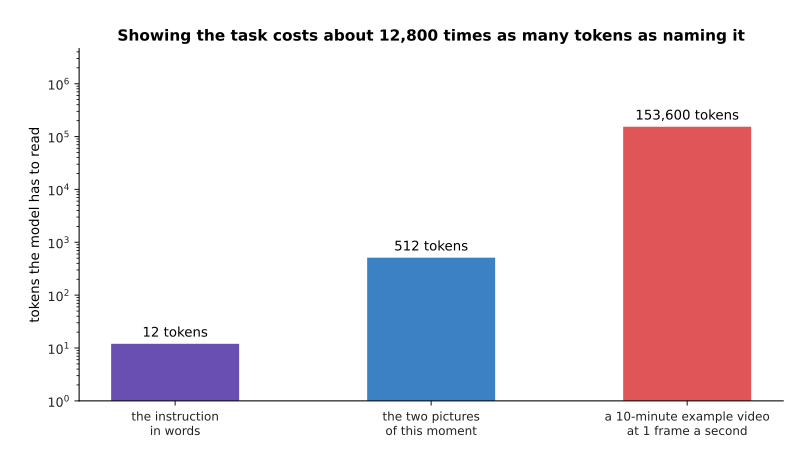
The instruction is 12 tokens and the two pictures of the current moment are 512 tokens, while a ten-minute example video kept at one frame a second is 600 frames, which is 153,600 tokens. That is about 12,800 times the instruction.

Attention compares every pair of tokens, so that sequence means about 23.8 thousand million pairs instead of 275,625. A model that reads an example therefore needs a body built to read very long sequences cheaply, which is a design decision taken before training starts.

What you get for that cost is a much more exact description of the task. The next picture measures how much, using the small flow head from section 4. Knowing only which task it is means the best single answer is the average chunk over the training data. Being shown an example of the movement means the head is told the ten actions just before the chunk.

A bar chart comparing the distance from the demonstrated chunk when only the task is
known against the distance when the ten preceding actions are
shown — A bar chart comparing the distance from the demonstrated chunk when only the task is known against the distance when the ten preceding actions are shown

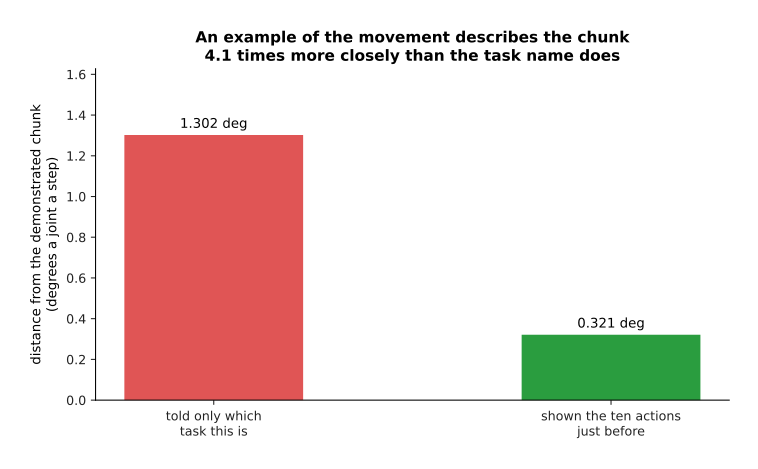
Knowing only which task it is leaves the best single answer 1.302 degrees a joint a step away from what was demonstrated. Being shown the ten actions just before the chunk brings that down to 0.321 degrees, which is 4.1 times closer.

That measurement is made on the simulated episodes of this page, so take the exact factor as an illustration rather than a result about real robots. What it does show honestly is the shape of the argument. An example of the movement describes what to do much more exactly than a name for the task does.

Reading an example also needs pretraining that makes reading an example something the weights can do. That is the same requirement that made few-shot prompting work for text, where a model is shown a few worked examples inside its input. It is why the models that do this are built for it from the start rather than adapted to it afterwards.

Skild S1, announced in August 2026, is the model that made this claim for manipulation. It is shown one video of a task lasting up to ten minutes, and it then performs the task with no fine-tuning. The company reports the two numbers in the next picture.

A bar chart of two reported success rates: 66 per cent when the model is shown one
example video, against 9 per cent when it is told the task in
words — A bar chart of two reported success rates: 66 per cent when the model is shown one example video, against 9 per cent when it is told the task in words

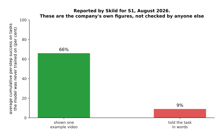
Skild reports 66 per cent success on tasks never seen before, against 9 per cent for models prompted with words, and reports that one video did the work of about 380 episodes of post-training.

Those figures should be read with care, and three facts decide how much weight to put on them. First, the comparison between 66 and 9 per cent is an average of cumulative per-step success rather than of whole tasks completed, so a task that is half finished still scores something, and that makes a long task look better than it was. Second, no architecture, no parameter count and no independent evaluation has been published. Third, the model is available only to commercial partners, so none of it can be checked on your own arm.

The idea belongs on this page anyway, because it separates two things this chapter has treated as one. A model's capability is held in its weights, but the task it performs does not have to be. Once the task arrives as input, teaching a robot something new stops being a training problem and becomes a recording problem, and that is a different kind of engineering from everything else in this book.

The next book works through what each route costs, and measures the trade-off on a worked example, in prompting with a demonstration.

9. Where to read next#

World models is the next page, and it covers models that predict what will happen next rather than reacting to what is there now.
Diffusion and flow policies holds the generative machinery the action head of section 4 is built from.
Fine-tuning and adapters explains catastrophic forgetting in full, which is what co-training exists to solve. It also covers where section 8's video prompt belongs, because showing a model an example changes none of its weights.
Running and evaluating a model takes section 7's latency arithmetic further and says how to test a policy honestly.
Vision-language-action models in the next book is the catalogue for this family, with the named models and their costs.
Vision-language models is the catalogue for the body these models are built from.

10. Using it in Python#

Section 3 measured what binning does to an action, and section 4 measured what a flow head does instead. Both are a few lines of real code. The lines below use NumPy and PyTorch, so that you can see that binning is arithmetic rather than a library, and that the head is an ordinary small network. No library gives you a whole vision-language-action model as one call, so this shows the output end, which is the part that differs between designs.

import numpy as np
import torch
from torch import nn

# Section 1: a chunk is CHUNK steps by ACTION_DIM numbers.
CHUNK, ACTION_DIM, BINS = 10, 7, 256
rng = np.random.default_rng(0)
chunks = rng.normal(0.0, 0.02, (64, CHUNK, ACTION_DIM))   # stand-in for recorded actions

# Section 3: the range comes from the data, then every number becomes a whole number.
lo = np.percentile(chunks.reshape(-1, ACTION_DIM), 1.0, axis=0)
hi = np.percentile(chunks.reshape(-1, ACTION_DIM), 99.0, axis=0)
z = np.clip(2.0 * (chunks - lo) / (hi - lo) - 1.0, -1.0, 1.0)
ids = np.clip(((z + 1.0) / 2.0 * BINS).astype(int), 0, BINS - 1)   # the action tokens
back = (ids + 0.5) / BINS * 2.0 - 1.0
rebuilt = (back + 1.0) / 2.0 * (hi - lo) + lo
print('tokens per chunk:', ids.size // len(chunks))                # 70
print('worst rounding, degrees:',
      round(float(np.degrees(np.abs(rebuilt - chunks).max())), 4))

# Section 4: the head is a small network that predicts a direction to walk in.
head = nn.Sequential(nn.Linear(CHUNK * ACTION_DIM + 1 + 1024, 256), nn.ReLU(),
                     nn.Linear(256, 256), nn.ReLU(),
                     nn.Linear(256, CHUNK * ACTION_DIM))
print('weights in the head:', sum(p.numel() for p in head.parameters()))

def sample(context, steps=8):                 # context is the model's last token
    x = torch.randn(len(context), CHUNK * ACTION_DIM)
    for k in range(steps):                    # section 4's walk, in equal steps
        t = torch.full((len(context), 1), k / steps)
        x = x + (1.0 / steps) * head(torch.cat([x, t, context], dim=1))
    return x.reshape(-1, CHUNK, ACTION_DIM)

print('chunk shape from the head:', tuple(sample(torch.zeros(4, 1024)).shape))

PyTorch gives you the layers, the gradients and the optimiser. A library such as Hugging Face transformers gives you the vision-language model that would supply the 1,024-number context in the last line. What no library decides is everything this page has been about. You choose the range the bins cover, which section 3 showed costs millimetres while the number of bins costs almost nothing. You choose between the two output styles, which section 4 showed is worth about ten times in speed. And you choose the mixture of robot and web data, which section 5 showed is the difference between keeping and losing what the model knew.

The subtle line is the walk inside sample. It starts from random numbers and takes equal steps in a direction the head predicts, and the number of steps is the setting measured in section 4. Training that head needs the flow-matching loss described on flow matching and other generators, which is a few lines more: draw a random list, mix it with a real chunk in some proportion, and train the head to predict the difference between them.

None of this code is the hard part. The hard part is collecting the demonstrations, and section 7 says why: what the model can do is set almost entirely by where the objects were when somebody recorded them.