Pretraining and Adapting — Scale, data and compute

The page before this one, self-supervised pretraining, showed where the training signal comes from when nobody writes labels. It ended with a frozen backbone that a few hundred labelled examples could be built on. However, it did not say what making that backbone costs. This page says what it costs, measured in machines, in memory, in arithmetic and in human time. Those costs are the reason almost nobody pretrains a model and almost everybody starts from one that somebody else pretrained.

This page answers five questions in order. What is the machine that training runs on, and why does it suit this work? What does one parameter cost to store? What does training need on top of the parameters, and why is that several times more than running the finished model? How is a whole training run measured, and how long does it take? And, given a budget, how should that budget be split between a bigger model and more data? The last section is about the data itself, which is where robotics differs from everything else, because every robot example costs a person time at a real arm.

The reader is assumed to have read two earlier pages. The shape of the numbers explains what a matrix multiply is and what float32 and bfloat16 mean. The training loop explains gradients and the optimiser. Every number here is worked out in docs/diagrams/pretraining_and_adapting_1.py. The model, the accelerator, the mixture of data and the scaling formula are example configurations written for this page and stated in full. None of them is a measurement of a real product.

Contents#

What a graphics processing unit does
What one parameter costs to store
What training needs on top of the parameters
Measuring a run in floating-point operations
Scaling laws, and what they let you plan
The data, and why the robot kind is scarce
Where to read next
Using it in Python

1. What a graphics processing unit does#

The first of the five questions above is about the machine. Training runs on a graphics processing unit, usually shortened to GPU. A GPU is a chip that was built first for drawing games, and that was then kept for neural networks because it turned out to suit them.

To see why it suits them, compare it with an ordinary central processing unit, or CPU. A CPU has a few very capable cores, and each core does one thing at a time, very quickly. A GPU instead has thousands of simple arithmetic units, and they all do the same kind of sum at the same time on different numbers. That arrangement only helps if your work can be cut into thousands of identical pieces that do not need to talk to each other.

A matrix multiply can be cut that way exactly, which is why this hardware fits. Every cell of the answer is worked out by running along one row of the first grid and one column of the second grid, multiplying the pairs and adding them up. No cell needs any other cell's result. The picture below shows one small multiply, with one row, one column and the cell they produce highlighted.

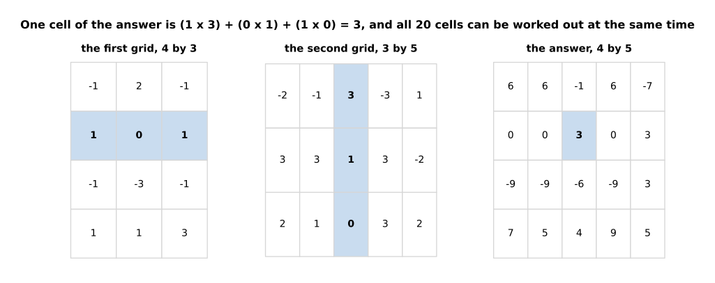
Three grids of small whole numbers, with one row of the first, one column of the second, and the resulting cell of the answer highlighted

The cell in row 2 and column 3 is (1 x 3) + (0 x 1) + (1 x 0) = 3. The whole 4 by 5 answer is 4 x 5 x 3 = 60 multiply-and-add pairs.

Because no cell needs any other cell, those 60 pairs can be shared out among as many workers as you have. The chart below counts how many steps the work takes, one after another, for three numbers of workers.

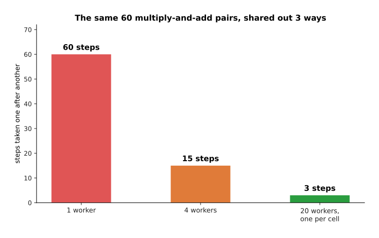
A bar chart of steps taken one after another: 60 steps with 1 worker, 15 with 4 workers and 3 with 20 workers

One worker takes 60 steps, four workers take 15, and twenty workers, one for each cell of the answer, take 3.

Make the grids bigger and the two counts move further apart, in a way that favours this hardware. Multiplying two grids of 1,024 by 1,024 takes 2.147 thousand million operations, spread over 1.049 million cells that can all be worked out at once, so each piece of work is 2,048 operations long. At a side of 16,384 it is 8.796 million million operations across 268.4 million independent cells.

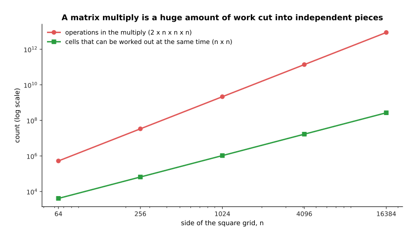
Two lines on a logarithmic chart: operations rising as the cube of the side, and independent cells rising as the square

The work grows as the cube of the side while the number of pieces it can be cut into grows as the square, so bigger multiplies both need more arithmetic units and can use them.

There is a second reason, and this one is about memory rather than arithmetic. Fetching a number from the chip's memory is slow compared with multiplying it. So what matters is how much arithmetic each fetched byte pays for. A matrix multiply of side 1,024 does 341 operations for every byte fetched, and at side 16,384 it does 5,461. Adding two grids together does 0.17 at every size, because it touches each number once and is then finished with it.

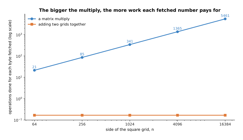
Two lines on a logarithmic chart: operations per byte fetched, rising steeply for a matrix multiply and flat at 0.17 for adding two grids

A big matrix multiply pays for each fetched byte many times over, while adding two grids touches each number once and then waits for memory again.

This has a direct consequence for how a model is run. Take one layer of 4,096 by 4,096 weights, which is 33.6 megabytes at two bytes a weight. The batch is the number of inputs put through the layer at the same time. Putting a single row of input through that layer takes 0.1 microseconds of arithmetic and 16.8 microseconds of fetching the weights, so the arithmetic units are idle 99 per cent of the time. The arithmetic only takes as long as the fetching at a batch of 256, and at a batch of 1,024 the arithmetic takes 85.9 microseconds against 25.2 for the fetching.

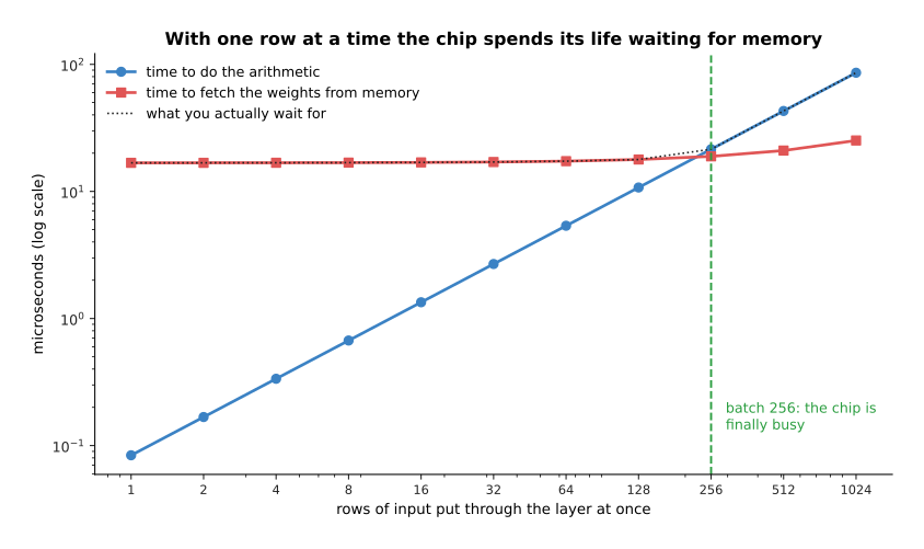
Two lines crossing on a logarithmic chart: arithmetic time rising with batch size, and weight-fetching time almost flat

With one row at a time the weights are fetched for almost nothing, and only at a batch of 256 does this layer spend more time on arithmetic than on memory.

That is why training uses large batches, and it is also why serving a model to one user at a time is wasteful. The next section looks at what those weights cost to hold in the first place.

2. What one parameter costs to store#

The last section counted operations, and this one counts bytes. The starting point is that a parameter is just a number, so its cost is the size of the number format it is kept in.

The example model used from here on is a transformer of 32 blocks with a width of 4,096 and a vocabulary of 128,000 tokens. Its parameter count follows from that shape alone. The attention parts hold 2.15 thousand million parameters, the feed-forward parts hold 4.29 thousand million, and the embedding table holds 0.52 thousand million, which is 6.97 thousand million in all. The chart below shows that split for three model shapes, with each bar stacked into its three parts.

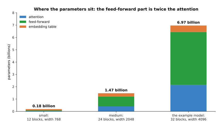
A stacked bar chart of parameters by part for three example model shapes, with attention, feed-forward and embedding table stacked in each bar

A small model of 12 blocks and width 768 has 0.18 thousand million parameters, and one of 24 blocks and width 2,048 has 1.47 thousand million. In every shape the feed-forward part holds twice what attention holds.

Multiplying the parameter count by the bytes of the number format gives the memory. At float32, which is four bytes a number, the example model needs 27.9 gigabytes before anything else is counted. At bfloat16, two bytes, it needs 13.9. At int8, one byte, it needs 7.0. At int4, half a byte, it needs 3.5.

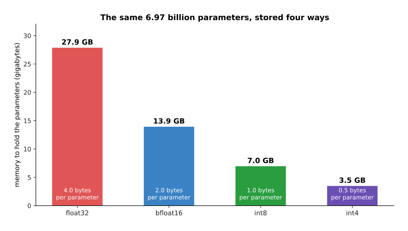
A bar chart of 27.9, 13.9, 7.0 and 3.5 gigabytes for the four number formats float32, bfloat16, int8 and int4

The same 6.97 thousand million parameters cost 27.9 gigabytes or 3.5 gigabytes, depending only on how many bits each one is kept in.

Fewer bits are not free, because a format with fewer bits rounds harder. To see why, look at how the bits of a number are divided up. A floating-point number is stored in three parts: one sign bit, then some exponent bits that say how big or how small the number is, then some fraction bits that say how finely it is rounded.

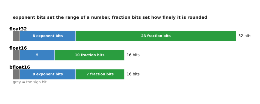
A diagram of three rows of coloured bit blocks, showing float32 as 1 sign bit plus 8 exponent bits plus 23 fraction bits, float16 as 1 plus 5 plus 10, and bfloat16 as 1 plus 8 plus 7

bfloat16 keeps all eight exponent bits of float32 and drops sixteen of the twenty-three fraction bits. So bfloat16 can hold the same range of sizes as float32 while rounding much harder than it. float16 does the opposite trade: it gives up three exponent bits to keep ten fraction bits.

The script now stores five numbers in four formats and measures how far each stored value is from the true one, as a share of that value. float32 is out by a few parts in a hundred million. float16 is out by a few parts in ten thousand. bfloat16 is out by up to about four parts in a thousand, for the reason the bit diagram shows. All three of those formats keep the same relative accuracy whatever the size of the number, which is what makes them safe for training.

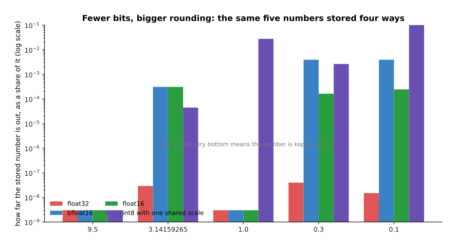
A bar chart on a logarithmic scale of the rounding error of five numbers stored in four formats

Storing 0.1 gives 0.1000000015 in float32 and 0.0996093750 in bfloat16. One shared int8 scale of 0.074803 turns the same 0.1 into 0.0748031496, which is a quarter out.

That last column shows the danger of whole-number formats. int8 does not store a number directly. It stores how many steps of a fixed size the number is, and the step size has to be agreed in advance. Here the step was set by the largest value in the set, so the smallest value lost a quarter of itself. Keeping a separate step for each part of the model is what makes int8 usable, and the page on making a model smaller and faster is about doing that properly.

The chart below turns these costs into the practical question, which is whether a model fits on one card at all. Each line is one number format, and the horizontal lines mark three example cards.

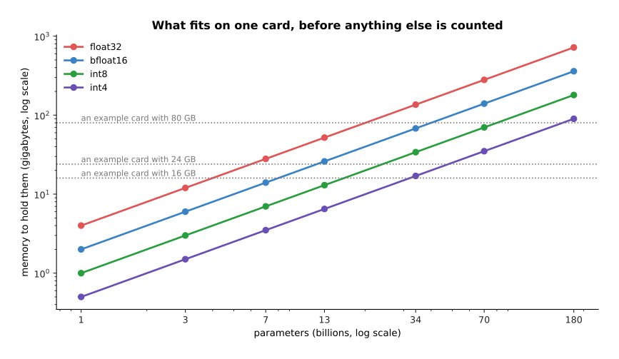
Four lines on a logarithmic chart of memory against parameter count, with horizontal lines marking example cards of 16, 24 and 80 gigabytes

A model of 7 thousand million parameters needs 28 gigabytes at float32 and 14 at bfloat16, so the format alone decides whether it fits on one card.

So far this is only the memory to hold a finished model and answer questions with it. Training needs considerably more, which is the next section.

3. What training needs on top of the parameters#

The memory counted in section 2 is only what a finished model needs to answer a question. Holding the parameters turns out to be the small part of training, because gradient descent has to keep several more numbers for every parameter.

There are four extra things to keep. First, the gradient of each parameter has to be stored while the backward pass runs. Second, the optimiser keeps running averages. The optimiser in almost every modern run is AdamW, and it keeps two running averages for each parameter. Third, the optimiser keeps those averages at float32, along with a float32 master copy of the parameter itself, because adding a tiny step to a bfloat16 number loses the step entirely. Fourth, every activation worked out on the way forward has to be kept until the backward pass has used it.

The chart below adds those five items up for one training step and puts the total beside the memory needed to simply run the finished model.

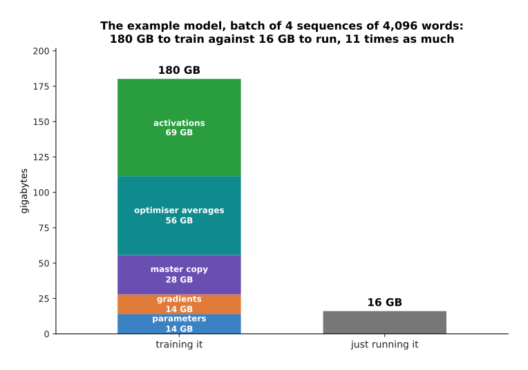
A stacked bar of five parts of training memory totalling 180 gigabytes, next to a single 16 gigabyte bar for running the model

Training the example model on four sequences of 4,096 words needs 14 gigabytes for the parameters, 14 for the gradients, 28 for the master copy, 56 for the two optimiser averages and 69 for the activations. That is 180 gigabytes in all, against 16 gigabytes for running it.

Those five numbers are worth reading twice. The parameters are 8 per cent of the total. The master copy and the two optimiser averages together are 46 per cent, which is more than five times what the parameters themselves cost. Training needs 11.2 times as much memory as answering with the finished model, which is why a model you can run on one card may need many cards to train.

The last line of the budget behaves differently from the others. The activations grow with the batch size, while everything else stays fixed at 111 gigabytes. At one sequence the activations are 17.2 gigabytes, and at 32 sequences they are 549.8 gigabytes. That is what sets the largest batch that fits.

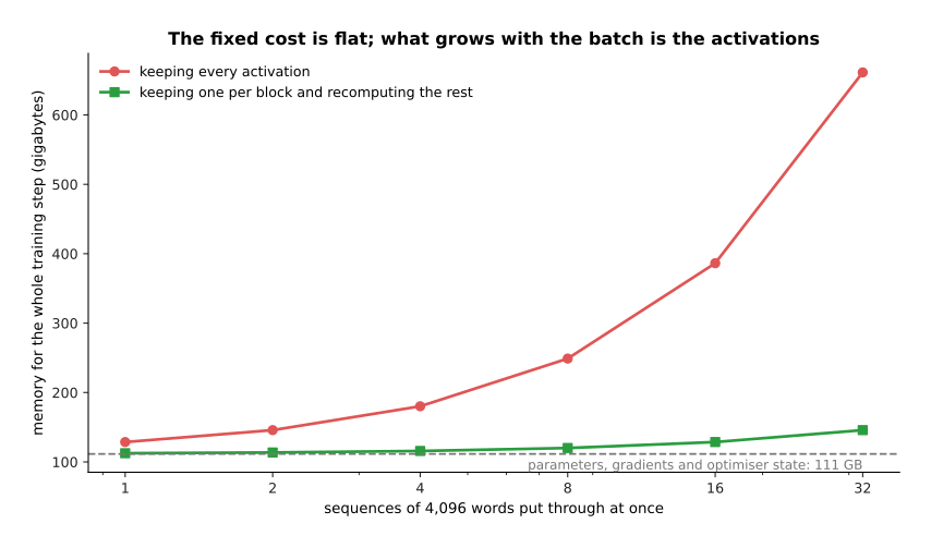
Two lines of total memory against batch size, one keeping every activation and one recomputing them, above a flat line at 111 gigabytes

The fixed cost of parameters, gradients and optimiser state is 111 gigabytes whatever the batch size, and only the activations grow with it.

There is a standard way of buying memory back. You throw most of the activations away during the forward pass and work them out again during the backward pass. Keeping one activation per block instead of all of them cuts the example budget from 180 gigabytes to 116, which is a saving of 36 per cent. The price is an extra forward pass, which raises the arithmetic of a step by about a third.

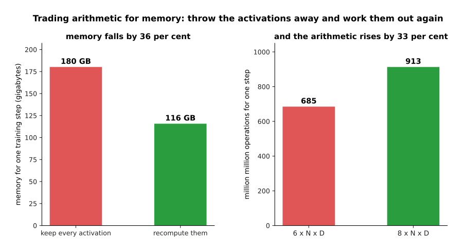
Two bar charts of the same choice: memory falling from 180 to 116 gigabytes, and arithmetic for one step rising by a third

Recomputing the activations trades 33 per cent more arithmetic for 36 per cent less memory, and it is switched on in almost every large run.

Counting sixteen bytes a parameter, which is the fixed part of the budget above, turns model size straight into a count of machines. The chart below does that for seven model sizes, using example cards of 80 gigabytes.

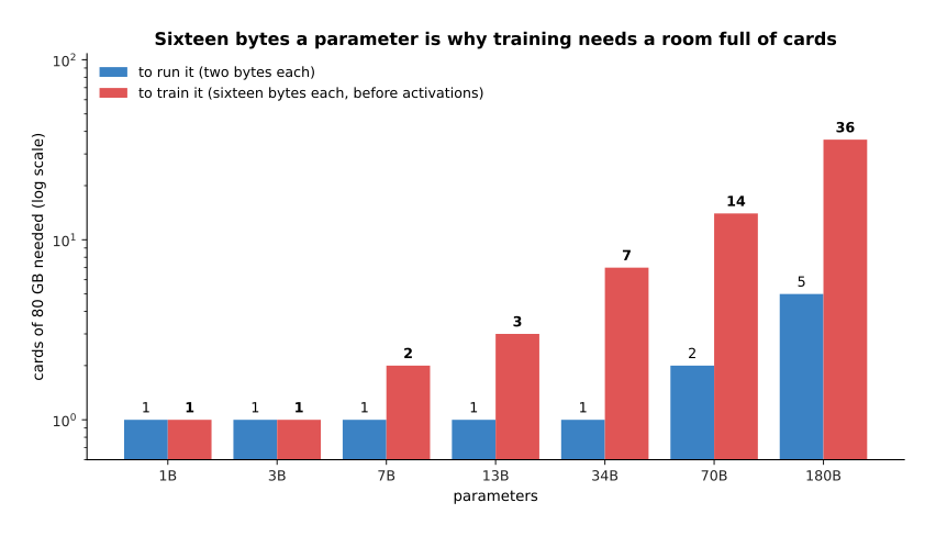
A grouped bar chart on a logarithmic scale of cards needed to run and to train, for seven model sizes

A model of 7 thousand million parameters fits on one card to run and needs two to train. One of 70 thousand million needs 2 cards and 14. One of 180 thousand million needs 5 cards and 36.

Memory decides whether a run is possible at all. How long it then takes is the next section.

4. Measuring a run in floating-point operations#

Section 3 decided whether a run fits in memory at all, and this section decides how long it takes. A floating-point operation, usually shortened to FLOP, is one multiply or one add on numbers with a decimal point. The size of a training run is measured by counting them, because that count does not depend on which machine you use.

The rule of thumb is simple enough to do in your head. Pushing one token through one parameter costs about two operations in the forward pass, because each parameter is multiplied by something and the result is added on. The backward pass costs about twice the forward pass, because it works out a gradient for the activations and a gradient for the weights. So a run over D tokens with N parameters costs about 6 x N x D operations in all.

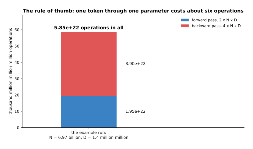
A stacked bar of forward and backward operations for the example run, totalling 5.85e+22

With 6.97 thousand million parameters and 1.4 million million tokens, the forward passes cost 1.95e+22 operations and the backward passes cost 3.90e+22, so the whole run costs 5.85e+22.

That number means nothing until it is divided by a machine. The example accelerator used here does 400 million million operations a second at full stretch. A real run keeps about 40 per cent of that busy, so it sustains 160 million million a second. One of them would take 12 years to finish the example run, which is why these runs are split across many accelerators at once.

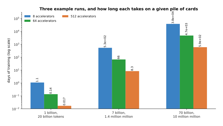
A grouped bar chart on a logarithmic scale of training days for three example runs on 8, 64 and 512 accelerators

The example run takes 532 days on 8 accelerators, 66 days on 64 and 8.3 days on 512. A run of 70 thousand million parameters over 10 million million tokens takes 593 days even on 512 accelerators.

Because the cost is a product of two numbers, many different pairs of model size and token count cost the same. Drawing lines of equal cost makes the choice visible. In the chart below the background colour is the cost and each black line joins the pairs that cost the same.

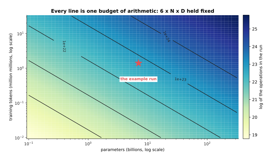
A heat map of 6 x N x D over model size and token count, with lines of equal cost drawn across it and the example run marked with a star

Every line is one budget of arithmetic held fixed, and the example run sits at 7 thousand million parameters and 1.4 million million tokens. Choosing a point on one of those lines is the subject of section 5.

The same rule prices answering as well as training. Producing one token with the finished model costs about 2 x N operations, which is 1.39e+10 here. So the training run costs as much as producing 4.2 million million tokens of answers, which is three times the number of tokens it was trained on. Training a model is a single large bill, and serving it is a small bill that never stops.

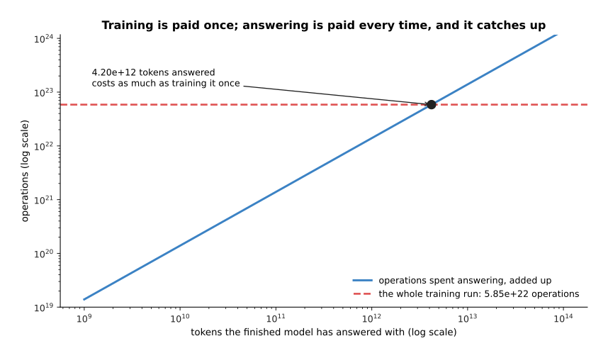
A rising line of cumulative serving cost crossing a flat line for the one-off cost of the training run

Answering costs as much as the training run once 4.2 million million tokens have been produced, and everything after that point costs more than training ever cost.

5. Scaling laws, and what they let you plan#

Section 4 left a question open. Given a fixed compute budget, which is the total number of operations you are willing to spend on one run, should that budget buy a bigger model trained on less data, or a smaller model trained on more? The answer comes from scaling laws, which are the measured relations between model size, data size, arithmetic and the loss the run ends at.

What people found, by doing many runs of different sizes, is that the loss falls smoothly and predictably as all three grow. They also found that the shape of the fall becomes a straight line when both axes are squashed logarithmically. The curves on this page come from a formula written for this page. The formula has that same shape without being anybody's measurement. It is a floor of 1.60, plus 500 divided by the number of parameters raised to the power 0.35, plus 500 divided by the number of tokens raised to the power 0.30.

The two panels below show the same curve twice: once with the loss on an ordinary axis, and once with the floor of 1.60 subtracted and both axes squashed.

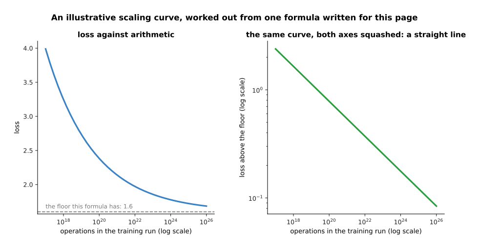
Two charts of the same curve: loss falling against arithmetic, and the same curve as a straight line once the floor is subtracted and both axes are logarithmic

In this illustrative formula, 7e+18 operations reach a loss of 2.802, 4.9e+20 reach 2.205 and 2.4e+24 reach 1.753. The fall becomes a straight line once the floor is subtracted.

Two things in that picture matter more than the exact numbers. First, the curve bends, so each further improvement costs more than the last one. Second, the curve has a floor, so no amount of arithmetic takes the loss to zero. Both of those things are true of the measured laws as well.

The second thing the laws say is that growing one of the three alone does not work, and that is the practical lesson. Hold the data at 10 thousand million tokens, and the loss in this formula cannot go below 2.100 however large the model gets. It is 2.454 at a thousand million parameters and still 2.171 at a hundred thousand million, so a hundred times the model has bought almost nothing.

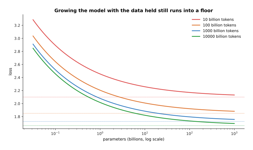
Four curves of loss against model size, one for each token budget, each one flattening onto its own floor

Each amount of data has its own floor: 2.100 for 10 thousand million tokens and 1.726 for a thousand thousand million. Growing the model while the data is held still brings the loss down onto that floor and no further.

So the budget has to be split between the two, and the split that the formula recommends grows both of them together. Multiplying the budget by ten multiplies the best model size by 2.89 and the best token count by 3.46.

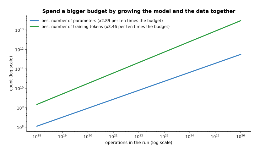
Two lines on a logarithmic chart, the best number of parameters and the best number of training tokens, both rising with the compute budget

Both the best model size and the best token count rise with the budget, and they rise at almost the same rate.

Because they rise at almost the same rate, the number of training tokens for each parameter stays nearly steady. The chart below follows that one number across a budget range of a hundred million to one.

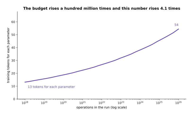
A line chart of the best number of training tokens for each parameter, rising slowly from 13 to 54 as the compute budget rises a hundred million times

The best number of tokens for each parameter drifts from about 13 at the smallest budget here to about 54 at the largest, while the budget itself rises by a factor of a hundred million.

The reason anyone cares about these laws is planning. A large run is expensive enough that you want to know roughly where it will end up before you start it. Because the relation is smooth, you can do several small runs, fit the line and read the answer for a run you have not done. The chart below does exactly that, using only runs between 1e+18 and 1e+21 operations to fit the line.

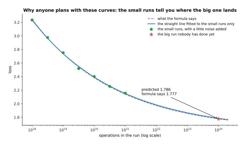
Seven small runs with a fitted straight line extrapolated to a point a thousand times further out

The line fitted to the small runs predicts a loss of 1.7856 at 1e+24 operations, where the formula itself gives 1.7768. That is an error of half a per cent.

One warning belongs with all of this. These laws predict the loss, which is how well the model guesses the next token. They do not predict whether the model can do the job you want. A better loss usually means a better model, and the word "usually" matters here: a run can reach a lower loss and still fail at your task.

6. The data, and why the robot kind is scarce#

Section 5 treated the data as a number of tokens, as if all tokens were alike. They are not, and the first thing that matters is how many of them are wrong. The script trains the same head on the same features three times: once with no wrong labels, once with one label in five wrong, and once with two labels in five wrong. Read the chart below as three curves of the same experiment with three levels of damage.

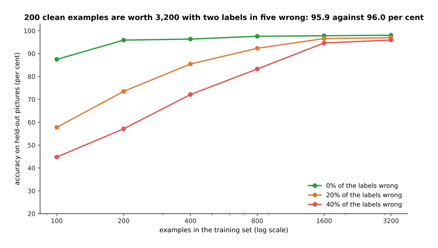
Three accuracy curves against training-set size, for clean labels, 20 per cent wrong labels and 40 per cent wrong labels

With 200 clean examples the head reaches 95.9 per cent, which is what 3,200 examples reach when two labels in five are wrong. At 400 examples the clean set reaches 96.4 per cent against 72.1 per cent for the damaged one.

The second thing that matters is how many of the examples are the same as each other. Text scraped from the web is full of duplicates, and a duplicate costs exactly as much to train on as a fresh example while teaching nothing. Removing them is called deduplication, which means finding and removing near-identical examples. It is one of the first things done to a newly collected set of data.

To show why, the script holds the training set at 1,600 examples and raises the share of them that are copies. Read the chart below from right to left: the set never changes size, but fewer and fewer of its examples are different from each other.

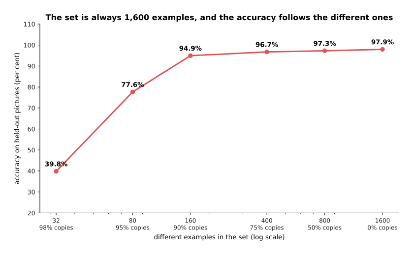
A line chart of accuracy against the number of different examples in a set that is always 1,600 examples, falling from 97.9 per cent to 39.8 per cent

Accuracy falls from 97.9 per cent with no copies, to 94.9 per cent when nine tenths of the set are copies, to 39.8 per cent when 98 per cent are copies and only 32 different examples are left.

The third thing that matters is which sources the tokens come from, and in what proportion. That choice is called the data mixture. The mixture is chosen rather than taken, because the amount of text available from each source has nothing to do with how much of it the model should read. The chart below shows an example mixture for a run of 1.4 million million tokens. For each source it draws two bars: how many tokens of that source exist, and how many the run actually reads.

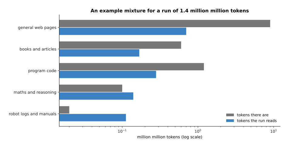
A horizontal bar chart on a logarithmic scale comparing tokens available with tokens read, for five sources of data

There are 9 million million tokens of general web pages and the run reads 0.7 million million of them. There are only 0.02 million million tokens of robot logs, and the run reads 0.112 million million.

Dividing the second bar by the first gives the number that actually matters, which is how many times each token of a source is read. The chart below shows that one number for each source, with a dashed line at one read each.

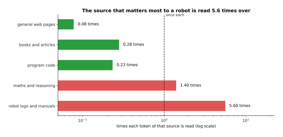
A horizontal bar chart on a logarithmic scale of how many times each token of each source is read, from 0.08 for web pages to 5.60 for robot logs

Each token of web pages is read 0.08 times, which means the run uses only a small part of what exists. Each token of robot logs is read 5.60 times, because that source makes up 8 per cent of the run while being the smallest source there is.

That last number is the whole problem of robotics stated once. The source you care about most is the smallest one, so it has to be read over and over, and reading the same example many times is how a model memorises instead of learning. Robot data is scarce for a reason that no amount of money removes quickly, which is that every example is a person sitting at a real arm. At 25 seconds to perform a task and 12 seconds to put the scene back, one person-hour yields 97 demonstrations.

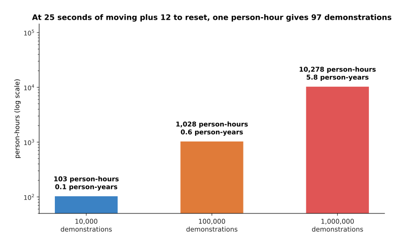
A bar chart on a logarithmic scale of the person-hours needed for 10,000, 100,000 and a million demonstrations

Ten thousand demonstrations cost 103 person-hours. A hundred thousand cost 1,028. A million cost 10,278 person-hours, which is 5.8 person-years of eight-hour days.

Four things are actually done about this, and each one gets examples more cheaply in exchange for examples that are less like the robot you will run on. The first is sharing data across robots, which is called cross-embodiment data. It means training on episodes recorded on other people's arms. It costs the time to convert those episodes into your own format, and it leaves you with data recorded on a body unlike yours. The second is simulation with randomised appearance and physics. It costs the time to build and randomise the scene, after which it produces episodes by the hundred thousand, and it leaves a gap between the simulator's physics and the real world. The third is synthetic data, which means examples generated by another model. It costs the time to set it up and to check what it produced, and it carries over the mistakes of the model that made it. The fourth is learning from video of people doing the task. It costs the least per example, because the video already exists, and it loses the most, because a human hand is not a gripper and a video holds no record of the forces.

The chart below prices those four against teleoperating a real arm, under example costings written for this page.

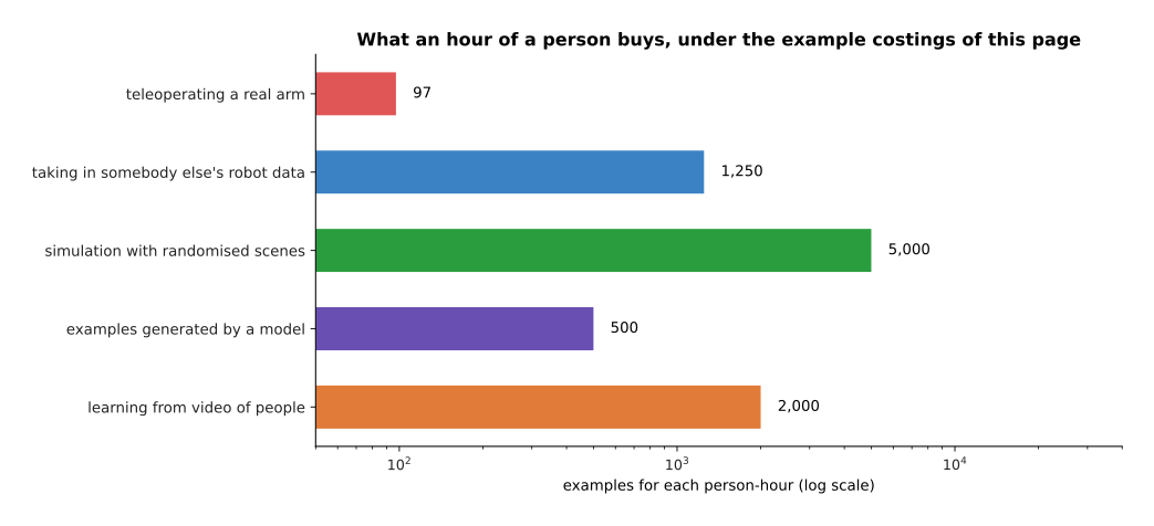
A horizontal bar chart on a logarithmic scale of examples bought by one person-hour, for five ways of getting robot data

Teleoperation gives 97 examples a person-hour, taking in somebody else's robot data gives 1,250, examples generated by a model give 500, learning from video gives 2,000, and simulation gives 5,000. Turned round, a hundred thousand examples cost 1,028 person-hours by teleoperation and 20 by simulation, and every cheaper route gives data that is further from the real arm.

None of this is a solved problem. The page on where the data comes from describes how real robot datasets are actually collected. The practical position today is that a robot model is pretrained on web text and pictures, where data is plentiful, and is then adapted with the small amount of robot data that exists. That adaptation is what the next page is about.

7. Where to read next#

Fine-tuning and adapters is the next page, and it shows how a pretrained model is adapted to one job without paying any of the costs on this page twice.
Making a model smaller and faster picks up section 2's int8 column and turns it into a model that fits on a robot's own computer.
Running and evaluating a model takes section 1's point about batches and memory and turns it into a latency budget for a real arm.
Vision-language-action models shows what is built from web pretraining plus the scarce robot data of section 6.
Where the data comes from is the catalogue page on real robot datasets, their sizes and how they were collected.
Hardware describes the arms and the computers that this arithmetic ends up running on.

8. Using it in Python#

Most of this page is arithmetic you can do without a library, and the first half of the program below does exactly that. The second half measures the thing that is easiest to get wrong, which is how much the optimiser adds to the memory. It does that by building one real transformer block, taking one step, and asking the optimiser what it is holding.

import torch
from torch import nn

# section 2: the parameter count of the example model, from its shape alone
def parameters(layers, width, vocab):
    return 12 * width * width * layers + vocab * width

n = parameters(layers=32, width=4096, vocab=128_000)
print(round(n / 1e9, 2))                       # 6.97 thousand million
for name, each in [("float32", 4), ("bfloat16", 2), ("int8", 1)]:
    print(name, round(n * each / 1e9, 1))      # float32 27.9 / bfloat16 13.9 / int8 7.0

# section 4: the arithmetic of a whole training run, 6 x N x D
tokens = 1.4e12
print(f"{6 * n * tokens:.2e}")                 # 5.85e+22

# section 3: what the optimiser adds, measured on one real block
block = nn.TransformerEncoderLayer(d_model=512, nhead=8, dim_feedforward=2048,
                                   batch_first=True)
small = sum(p.numel() for p in block.parameters())
print(small)                                   # 3152384

opt = torch.optim.AdamW(block.parameters(), lr=1e-4)
block(torch.randn(2, 16, 512)).sum().backward()
opt.step()
state = sum(v.numel() for s in opt.state.values()
            for v in s.values() if torch.is_tensor(v))
print(state, round(state / small, 1))          # 6304780 2.0

The first three prints are section 2 and section 4 with no library involved at all, because a parameter count follows from the shape of the model and the cost of a run follows from the parameter count. The formula 12 x width x width x layers is the attention and feed-forward parts of a standard block added together, and the vocabulary times the width is the embedding table.

The last two prints are the measurement. One real block of width 512 holds 3,152,384 parameters. After a single AdamW step the optimiser is holding 6,304,780 numbers of its own, which is 2.0 times the size of the model. Those are the two running averages of section 3. At float32 they come to eight bytes for every parameter, which is 31 per cent of the training budget. Add the float32 master copy, which is another four bytes a parameter, and the optimiser's whole state is the 46 per cent that section 3 counted.

What PyTorch will not tell you is any of the planning. It does not warn you that your batch is too small to keep the chip busy, that your model is too large for the data you have, or that half your training set is duplicates. Those are decisions, and sections 3 to 6 are how they are made: count the bytes before you start, count the operations, pick a point on the line of equal arithmetic cost, and look at the data you have before you buy more of it.