The page before this one, why the transformer won, ended with a machine that can read a very long piece of text and let every part of it look at every other part. That machine needs a very large amount of training data. It needs so much because it has hundreds of millions or billions of parameters, which are the numbers inside the model that training adjusts. A model with that many numbers to set needs an enormous number of training examples before it settles on good values for them.
So a question has been waiting since the start of this book. Training normally needs a right answer written down beside each example, and that written answer is called a label. If a person has to write a label for every training example, and writing one takes twenty seconds, where could enough labels possibly come from?
The answer is that for almost all of the training nobody writes them. Instead the data is arranged so that it asks the question and holds the answer at the same time. This is called self-supervision, because the training signal is taken out of the data rather than put there by a person. Training a model this way, on a very large collection of unlabelled data, before the model is pointed at any one job, is called pretraining. The invented job that the model is trained on is called a pretext task, which means a task nobody actually wants the answer to. Such a task is chosen because learning to do it forces the model to learn something worth having.
This page is for a reader who has already met a neuron, a layer, a loss, gradient descent and the transformer. It also assumes you have seen next-word prediction once already, on the page about training and running a transformer. By the end of this page you will understand four families of pretext task, you will have seen one of them worked out in full with real numbers, and you will know what you are left with when pretraining finishes.
Every number here comes from a program that really runs, in
docs/diagrams/pretraining_and_adapting_1.py. Its sentences are simulated, which
means they are generated from a tiny hand-written grammar rather than collected
from the world. Its pictures are simulated too, built from a few smooth patterns
with random noise added to every pixel. The models fitted to that data are real,
and every loss and accuracy quoted below is measured on data the model was not
fitted to.
Contents#
- Where the training signal comes from when nobody writes labels
- Next-word prediction, which you have already met
- Masked prediction: hide part of it and fill it in
- Contrastive learning, worked out with real numbers
- Self-distillation: agreeing with a slower copy of yourself
- What you are left with, and what it is worth
- Where to read next
- Using it in Python
1. Where the training signal comes from when nobody writes labels#
The problem is a problem of arithmetic, so the first thing to do is to count. Suppose you have four thousand short sentences. In the simulated collection of sentences used here, those four thousand sentences contain 33,320 words in total, and only 28 different words are ever used. A collection of text like this is called a corpus.
Now suppose a person reads each sentence and writes one answer beside it. That gives you 4,000 training signals. If writing one answer takes twenty seconds, the whole job takes 22.2 person-hours, where a person-hour means one person working for one hour.
Now take the same text and ask a different question of it. At every position in every sentence, cover the next word, ask the model to guess it, then uncover it and see whether the guess was right. There are 29,320 places in this corpus where that can be done. The first chart below compares those two counts, so read it as one bar for the answers a person writes and one bar for the answers the text already contains.
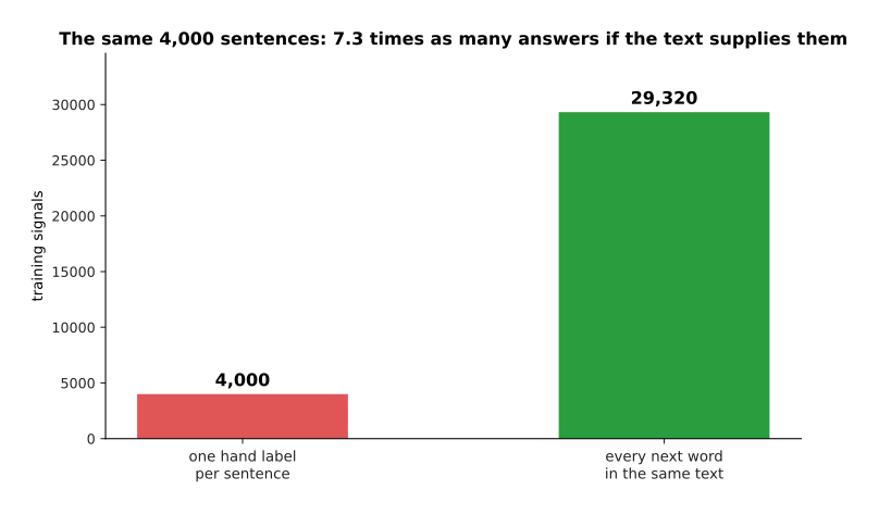
The same four thousand sentences give 4,000 answers if a person writes them and 29,320 if the text supplies them, which is 7.3 times as many.
The second chart compares the cost of those same two columns, measured in the time a person has to spend. Read it as the price of each bar in the chart above.
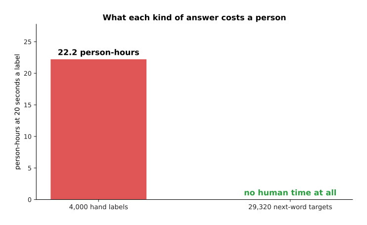
The hand-written answers cost 22.2 person-hours and the next-word answers cost nobody any time at all, because each answer was already sitting in the sentence.
The next picture shows where those free answers come from. It takes one sentence and writes out every training pair it contains. Each row shows the words the model is allowed to see on the left, and the word it must guess on the right.
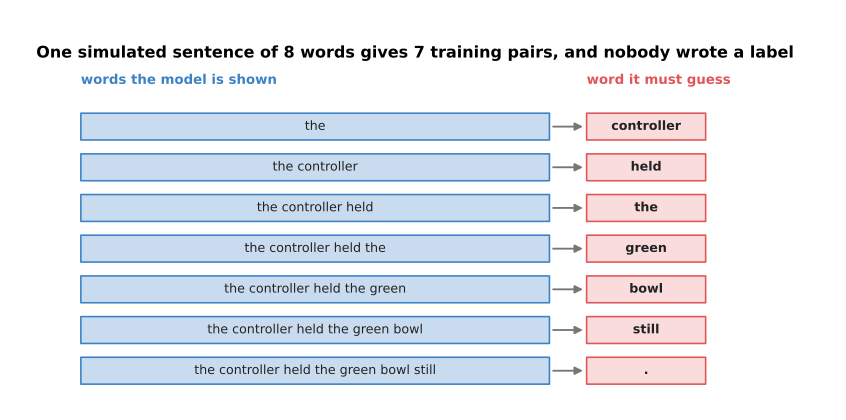
One simulated sentence of eight words becomes seven training pairs, and the answer in each pair was cut out of the sentence itself.
The same counting works for pictures, and for pictures the gap is even larger. A colour photograph of 224 pixels by 224 pixels holds 150,528 numbers, because each of the 50,176 positions carries three numbers, one for red, one for green and one for blue. If a person labels that photograph with the name of the object in it, the whole picture has bought one training signal.
Now cut the same picture into small squares of 16 pixels by 16 pixels. That gives a grid of 14 by 14, so 196 squares in all. The next picture shows what happens when three quarters of those squares are hidden.
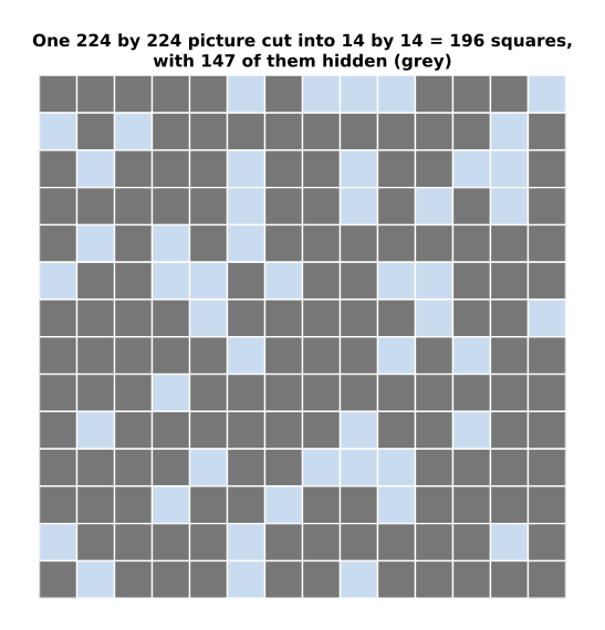
Hiding three quarters of the squares hides 147 of them and leaves 49 visible, so the model has 147 separate things to work out about this one picture.
The chart below counts the three ways of using that same picture. The bars use a logarithmic scale, which means each step up the axis multiplies the count by ten, so bars of very different sizes can be shown together.
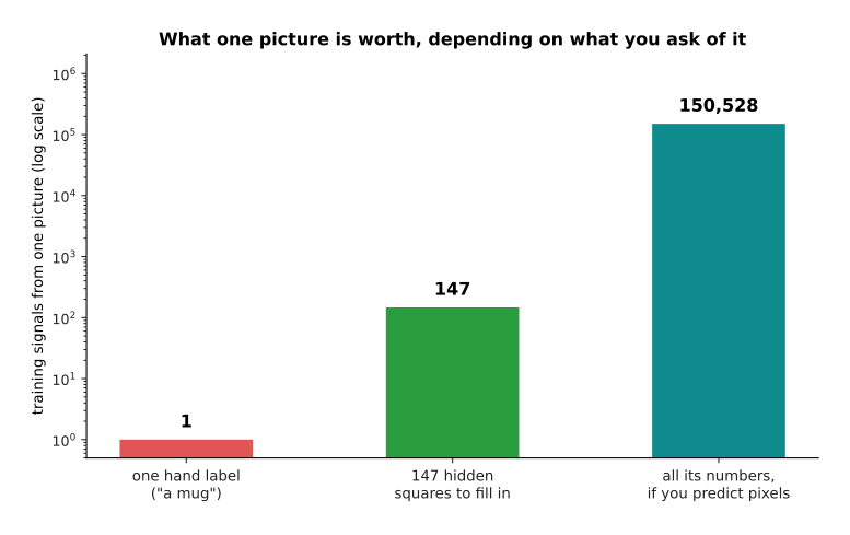
One picture is worth one hand label, 147 hidden squares to fill in, or 150,528 pixel values, depending on what you ask of it. Nobody wrote any of those 147 answers down.
So the recipe is always the same, and it has two steps. First, hide something the data already contains. Second, make the model produce the hidden thing from what is left. What changes between the four families of pretext task is what gets hidden. Next-word prediction hides the word that comes next. Masked prediction hides part of a picture or part of a sentence. Contrastive learning hides which caption belongs to which picture. Self-distillation hides nothing at all, and instead asks two different views of one object to produce the same answer. The rest of this page takes those four in order, starting with the one you have already met.
2. Next-word prediction, which you have already met#
The page on training and running a transformer showed next-token prediction as the way a language model is trained. A token is a piece of a word, as tokens and embeddings explained. Next-token prediction is one example of the general recipe above. It was chosen because text is a sequence, so the obvious thing to hide is what comes next. On this page the tokens are whole words rather than pieces of words, which keeps the arithmetic small.
The picture below shows one sentence and every job inside it. Each arrow starts at a position in the sentence and points at the word that the model must name there.
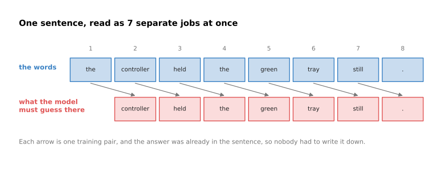
The eight words of one sentence are read as seven jobs at once, because at every position except the last one the model must name the word that comes next.
Now look at what this job forces the model to learn. The script fits four models to this corpus by gradient descent and measures each one on sentences it was not fitted to. The measure used is the loss from the score of being wrong, so a loss of 0 would mean the model gave the right word a probability of 1. Beside each loss the chart also prints what that loss would mean if the model were simply picking at random from that many equally likely words, which makes a loss easier to imagine.
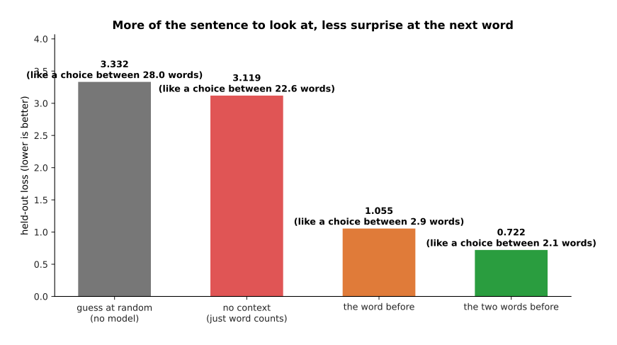
Guessing at random gives a loss of 3.332. Knowing only how often each word appears gives 3.119. Seeing the one word before the gap gives 1.055, and seeing the two words before gives 0.722.
Those four numbers are why this pretext task is worth anything. Learning only which words are common saves almost nothing, because the loss moves from 3.332 to 3.119. However, being allowed to look at the word before cuts the loss to 1.055, and looking at two words cuts it to 0.722. Each of those savings had to be paid for with real knowledge about the language. The model got that knowledge by being wrong on 23,488 training pairs and adjusting itself each time.
The next picture opens up two single positions and shows what the model believes at each of them. Each bar is one word, and the length of the bar is the probability the model gives that word.
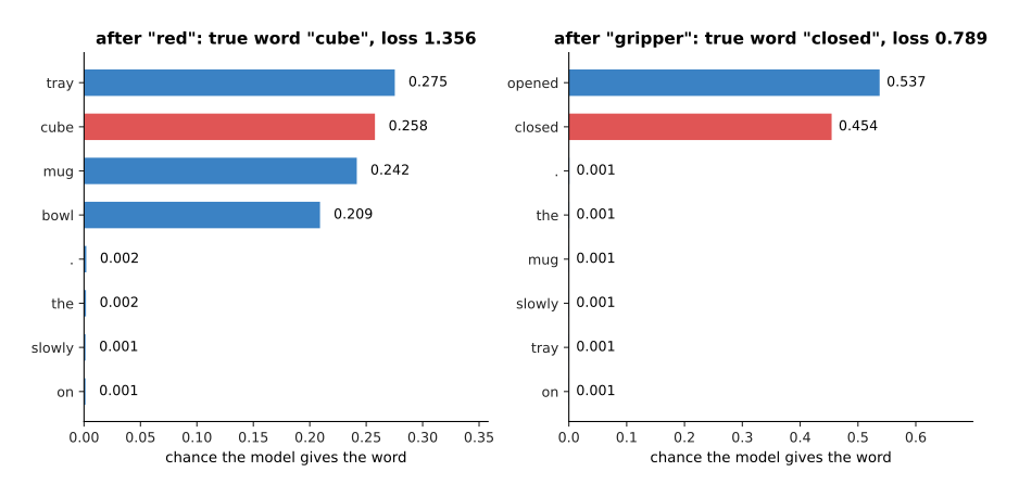
After the word "red" the model spreads its answer across the four objects, giving "tray" 0.275 and the true word "cube" 0.258. After the word "gripper" it gives almost everything to "opened" at 0.537 and "closed" at 0.454.
Read those two charts carefully, because they show two different rules that the model worked out on its own. After a colour word the model has learned that an object comes next, and it divides its answer between the four objects almost evenly. It does that because nothing in this corpus says which object is coming. A model that claimed to know would be wrong three times in four, and the loss would punish it for that. After "gripper" the model has learned that only two verbs ever follow. Nobody taught it either rule.
The next picture shows the two best models learning, step by step, over four thousand gradient steps.
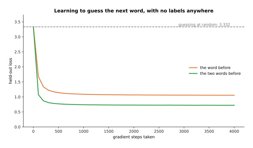
Both models start at the loss of random guessing, 3.332. The one-word model settles at 1.055 and the two-word model settles at 0.722.
At the scale of a real language model, this same job over a very large amount of text is what produces a model that can hold a conversation. That happens because guessing the next word well enough eventually requires knowing what words mean. The next section takes the same idea to data that is not a sequence.
3. Masked prediction: hide part of it and fill it in#
The method in section 2 needs an order, and a picture has no order. Nothing in a picture comes first, so covering what comes next does not transfer to pictures at all. What does transfer is the idea underneath it, which is to hide part of the input and make the model produce the hidden part from what is left. That idea is called masked prediction. The mask is the list of which parts are hidden.
The three panels below show one simulated picture at three stages of the same process: as it really is, with the hidden squares marked, and as the model sees it.
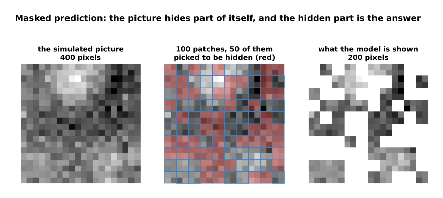
Each simulated picture is 400 pixels cut into 100 patches of 2 pixels by 2 pixels. Half the patches are hidden, so the model sees 200 pixels and must produce the other 200.
The model fitted here is the plainest one that can do the job. It is a set of weights that turns the 200 visible pixels into a guess at the 200 hidden ones, and it was fitted on 12,000 unlabelled pictures. What the model is asked for is the picture underneath the noise, not the noisy pixels themselves. The reason is that the noise in this simulated data is independent of everything else, so nobody can predict it. Measured against the noise-free picture, the fitted model is 0.264 per pixel out. A model that always answers with the average picture of the training set is 2.182 per pixel out. So learning the shape of a picture has cut the error by 88 per cent.
The next picture takes two test pictures the model has never seen and shows each one three times: as the model sees it, as the model fills it in, and as it really was.
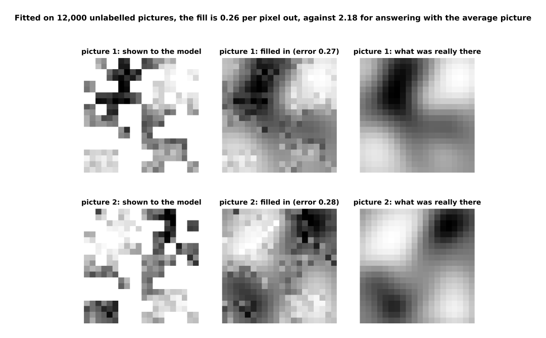
On both pictures the fill lands close to what was really there, with errors of 0.268 and 0.284 per pixel.
How much you hide decides how hard the job is. To show this, the script refits the same kind of model on 8,000 pictures at six different mask rates, where the mask rate is the share of the patches that are hidden.
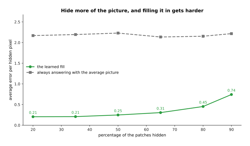
The error rises from 0.206 per pixel when a fifth of the patches are hidden to 0.743 when nine tenths are hidden, while the average-picture model stays near 2.2 at every rate.
Hiding very little makes the job easy in a way that is useless, because a patch can be copied from its neighbours without understanding anything about the picture. That is why real systems for pictures hide most of the image.
Masked prediction works on text as well, and there it differs from next-word prediction in one way that matters. When a model fills a gap in a sentence, it has the words on both sides of the gap available. The script fits two models to the same corpus: one that sees only the word before the gap, and one that sees the words on both sides. The second model has a held-out loss of 0.492 against the first model's 1.111.
The next picture takes one sentence with one word hidden and shows what each of those two models believes. Read the two charts as the same question answered with less information and with more.
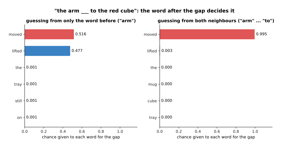
Knowing only that "arm" comes before the gap leaves the model split between "moved" at 0.516 and "lifted" at 0.477. Knowing that "to" follows the gap settles it at 0.995 for "moved".
That is the trade. Filling a gap from both sides is a better way to learn what a word means in its place, which is why models built to understand text are trained this way. However, it is useless for writing text one word at a time, because when you are writing there is nothing on the right yet. The next section leaves hidden parts behind.
4. Contrastive learning, worked out with real numbers#
Both methods so far hide part of one thing. Contrastive learning hides something else: which items belong together. You start with pairs that go together, such as a photograph and the caption written under it. Then you train two models at once. One model turns a picture into a short list of numbers, and the other turns a caption into a short list of numbers. The training makes the two lists of a matching pair point in the same direction, while the lists of things that do not belong together point in different directions.
A short list of numbers like that is a vector. How much two vectors point the same way is measured by their cosine similarity, which runs from +1 when they point the same way, through 0 when they are unrelated, to -1 when they point in opposite directions. Both of those words were explained on tokens and embeddings.
In the simulated data each item has a hidden content vector. The picture side and the caption side are two noisy views of that content vector, so the only thing the two sides share is the content. After training, take six items and work out the similarity of every picture against every caption. The grid below shows those thirty-six numbers. Read a row as one picture scored against all six captions, and read the boxed cell on the diagonal as the pair that really belongs together.
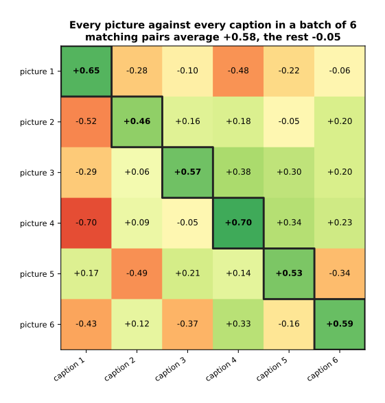
The six matching pairs average +0.58 and the thirty non-matching pairs average -0.05. In every row the largest number is the matching one.
Now comes the important part, which is where the training signal comes from. Take one row of that grid, the row for picture 3. Its six similarities are -0.287, +0.056, +0.570, +0.375, +0.301 and +0.199. Divide all six by a small number called the temperature, which is 0.1 here. That gives -2.87, +0.56, +5.70, +3.75, +3.01 and +1.99. Then push those six numbers through softmax, which is the function that turns a list of numbers into a list of probabilities that add up to
- The result is 0.000, 0.005, 0.805, 0.115, 0.055 and 0.020. So the model gives its own caption a probability of 0.805. The loss for that row is the usual one, the negative logarithm of 0.805, which is 0.216. Picking at random from six captions would have given a loss of 1.792.
The picture below shows that row twice: once as the raw similarities, and once as the probabilities they turn into. Read the left chart as the measurement and the right chart as the same measurement after dividing by 0.1 and applying softmax.
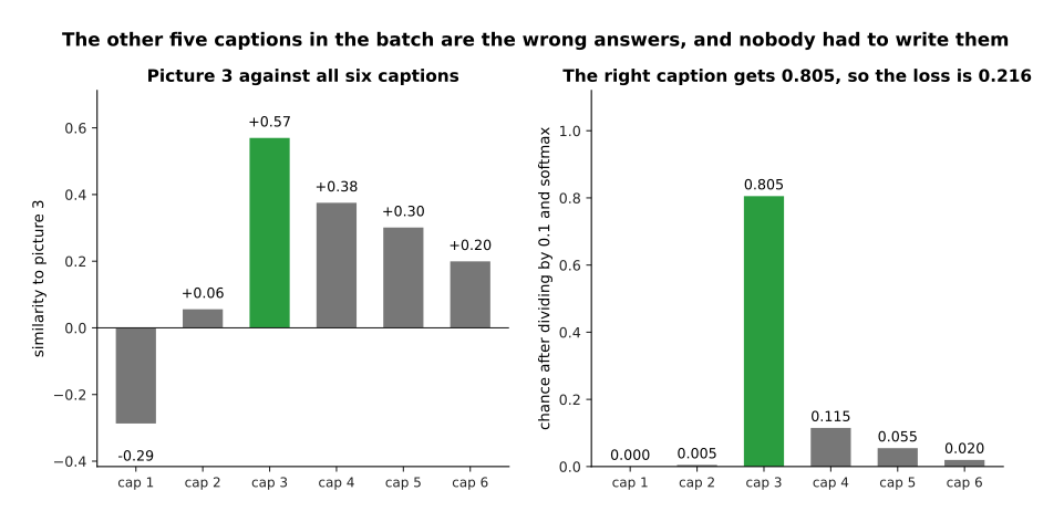
Picture 3 picks its own caption out of the six and gives it 0.805, so the loss for that row is 0.216.
This is why the other examples in the batch matter so much. The five other captions are the wrong answers that the right one has to beat, and they are called the negatives. Nobody wrote those down either, because they are simply whatever else happened to be in the batch. The whole batch is scored this way twice, once with each picture choosing a caption and once with each caption choosing a picture, and the average of the two is what gradient descent is given.
The next picture shows the same six pairs measured before training and after training. The two grids are the same measurement at two moments, so compare the boxed diagonal in one with the boxed diagonal in the other.
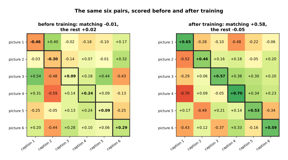
Before training the matching pairs average -0.01 and the rest average +0.02, so a matching pair is no more alike than any other pair. After training the matching pairs average +0.58 and the rest average -0.05.
The chart below shows the loss itself falling as the training runs.
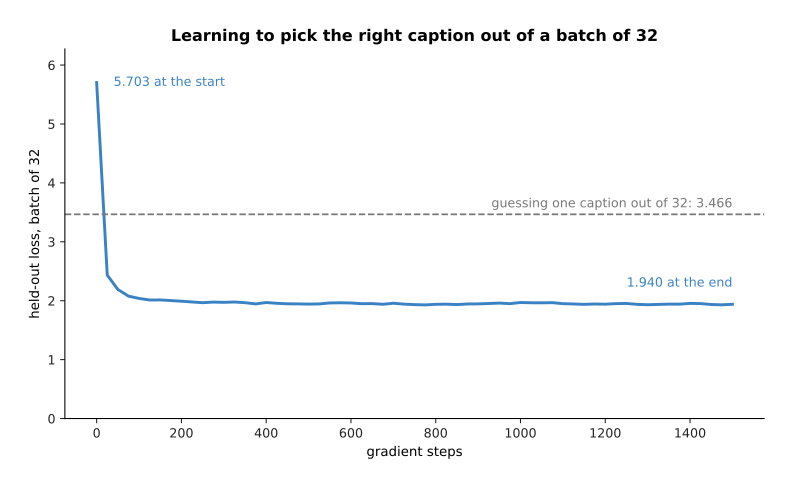
The held-out loss falls from 5.703 before training to 1.940 after it, and guessing at random from a batch of 32 would give 3.466.
Two choices control this method, and the first is the batch size. The batch size decides how many wrong answers each right one has to beat, so a bigger batch is a harder question. The chart below measures the trained model at seven batch sizes and compares each one with random guessing.
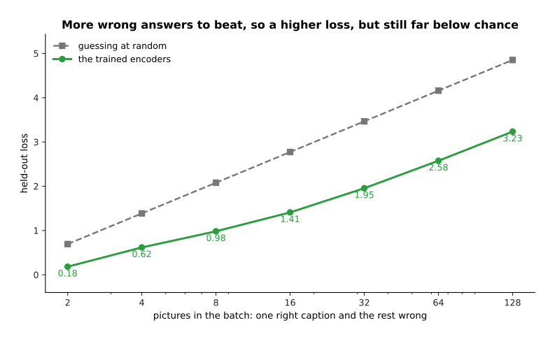
The trained model's loss rises from 0.182 with a batch of 2 to 3.234 with a batch of 128, while the loss of random guessing rises faster still, from 0.693 to 4.852.
The second choice is the temperature, which decides how sharply small differences in similarity are treated. A small temperature makes the model commit hard to its best guess, and a large one makes it spread its answer out. Sweeping the temperature over nine values gives the curve below.
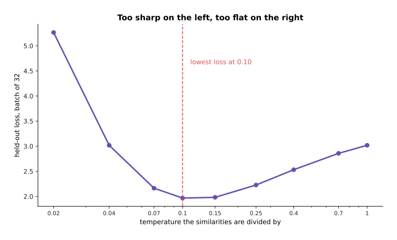
The lowest held-out loss is 1.967 at a temperature of 0.10. The loss rises to 5.265 at 0.02 and to 3.019 at 1.00, so there is one best value and it is not at either end.
This is how the CLIP family of models is trained, where CLIP stands for contrastive language-image pretraining. Those models are trained on a very large number of pictures together with the text that happened to be beside them on the web. What this method gives you is worth saying plainly, because a later chapter depends on it. Pictures and words end up in the same space of vectors. That means you can name an object the model was never given a label for: you write the name as a sentence, turn that sentence into a vector, and see which picture it points at. That is what open-vocabulary vision is built on, and it is why a robot can be asked for "the blue mug" when nobody has ever trained a blue-mug detector.
5. Self-distillation: agreeing with a slower copy of yourself#
Contrastive learning needs pairs of two different kinds of thing, such as a picture and a caption. For pictures alone there are no captions to use. Self-distillation removes that need. It cuts two pieces out of the same picture, pushes both pieces through the same network, and trains the network so that what it says about one piece matches what a slower copy of itself says about the other piece. A piece cut out of a picture is called a crop. The slower copy is called the teacher, the network being trained is called the student, and the teacher's weights are the student's weights smoothed over the last hundred steps or so.
The four panels below show one simulated item. The first two panels are the same object photographed twice under different lighting, with the crop marked on each. The third panel shows the two crops on their own, and the fourth shows the part of the picture that the two photographs have in common.
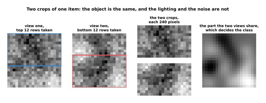
Each crop is twelve rows of a twenty by twenty picture, and the two crops share four rows. Across the batch, the part that says what the item is varies by 1.46 per pixel, while the lighting that differs between the two views varies by 2.41 per pixel.
The model's answer is neither a picture nor a word. It is a share given to each of eight directions called prototypes. The prototypes start as random directions and are learned along with everything else, so the answer says something like "this crop belongs mostly to prototype 7". The teacher's answer is made sharper than the student's, by dividing by a smaller temperature. Before that sharpening, a running average of the teacher's recent scores is subtracted from its scores.
The two charts below show one item. The left chart is the student looking at crop one, and the right chart is the teacher looking at crop two.
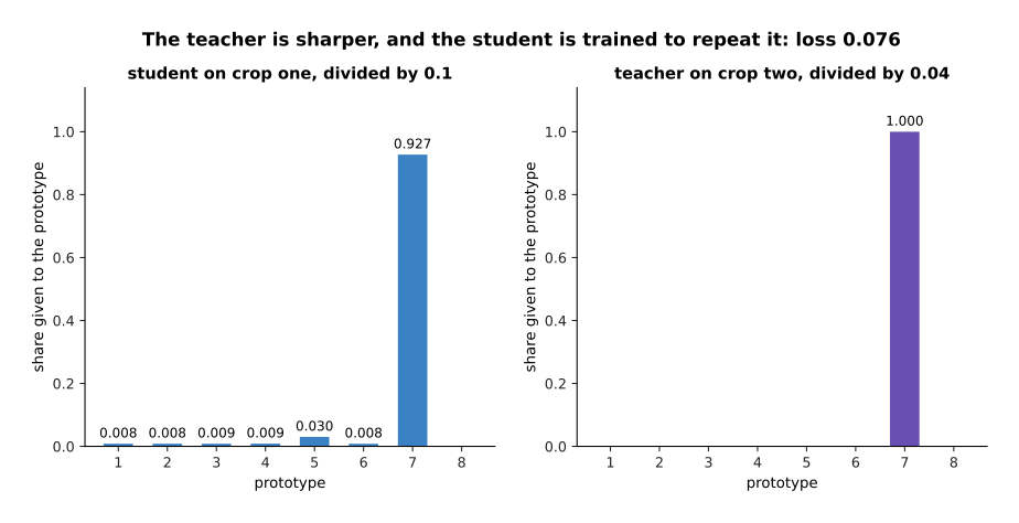
The student puts 0.927 on prototype 7, and the sharper teacher puts almost all of its answer on the same prototype, so the loss for this item is 0.076.
That subtraction and that sharpening are both necessary. There is an obvious way to satisfy the rule "agree with yourself", which is to give every picture the same answer. That failure is called collapse. Collapse would make the loss zero while teaching the model nothing. Subtracting the running average pushes the teacher away from whichever prototype it has been favouring, and the sharpening stops the answers from drifting into one flat spread where every prototype gets the same share.
The chart below measures the loss between the student's answer and the teacher's answer as the training runs.
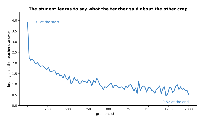
The student learns to say what the teacher said, so the loss falls from 3.91 at the start to 0.52 at the end.
The next chart checks that collapse did not happen. It measures how spread out the answers are across the eight prototypes, with two reference lines drawn in: a value of 0 means every picture got the same answer, and 2.079 means all eight prototypes were used equally.
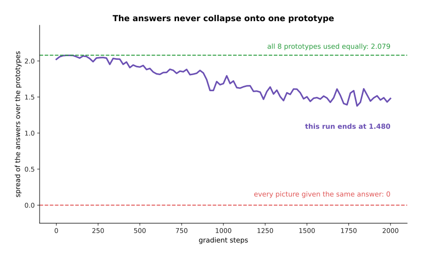
The answers stay spread out, ending at 1.480, which is far above the 0 that collapse would give.
The chart below asks the question that actually matters. It takes items the model never trained on, cuts two crops from each, and counts how often the two crops are given the same prototype.
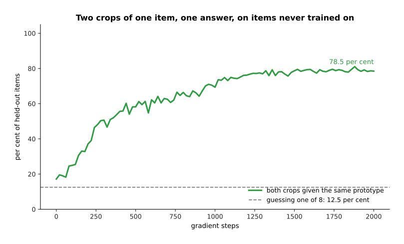
On items it never trained on, the two crops are given the same prototype 78.5 per cent of the time, against 12.5 per cent for guessing one of eight at random.
The point of all this is what happens to the sixteen numbers the network works out on the way to its answer, because those numbers are the thing worth keeping. The two charts below count pairs of crops by how similar their sixteen numbers are, once before training and once after. In each chart, one colour is two crops of the same item and the other is crops of two different items.
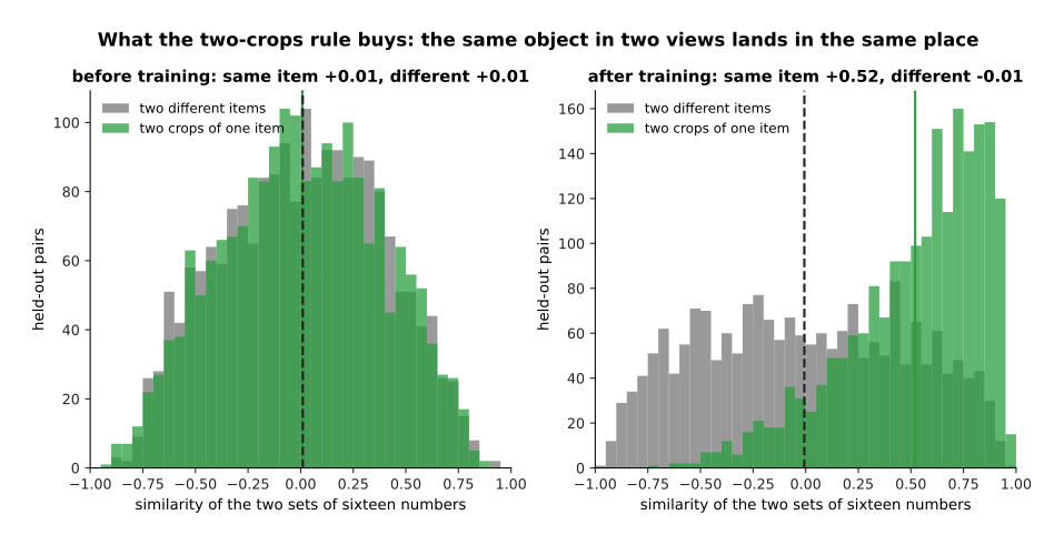
Before training, two crops of one item are no more alike than two crops of different items, at +0.008 against +0.010. After training they sit at +0.520 against -0.006, so the two groups have separated.
This is how the DINO family of vision models is trained, and the name is short for self-distillation with no labels. It gives you a network whose output ignores what differs between two views of one object and keeps what does not differ. That output is the next section's subject.
6. What you are left with, and what it is worth#
The four methods of sections 2 to 5 all end in the same place, and that place is not a model that does a job anybody wants. Each one ends with a representation, which is a way of turning a raw input into a shorter list of numbers that says what is in it. The part of the network that does that turning is called the backbone. The job you actually care about is then done by a head, which is a small network that reads those numbers and gives the answer you want. When the backbone's weights are left exactly as pretraining made them, and only the head is trained, the backbone is said to be frozen.
The picture below follows one real test picture through both parts, from left to right, with the numbers this page's demonstration really produces.
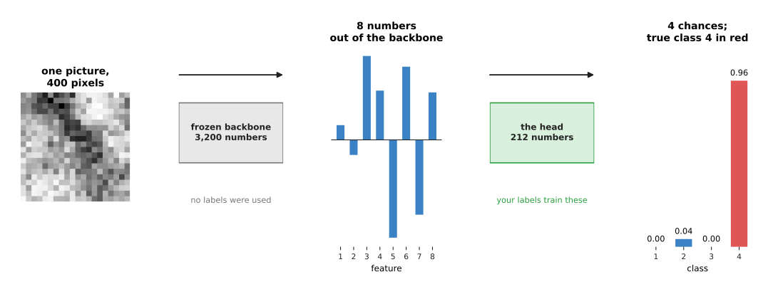
The frozen backbone turns 400 pixels into 8 numbers without any label having been used, and the head turns those 8 numbers into a probability for each of the four classes, giving 0.96 to the true class.
The chart below counts the numbers in each part. It uses a logarithmic scale, because the three counts are very different in size.
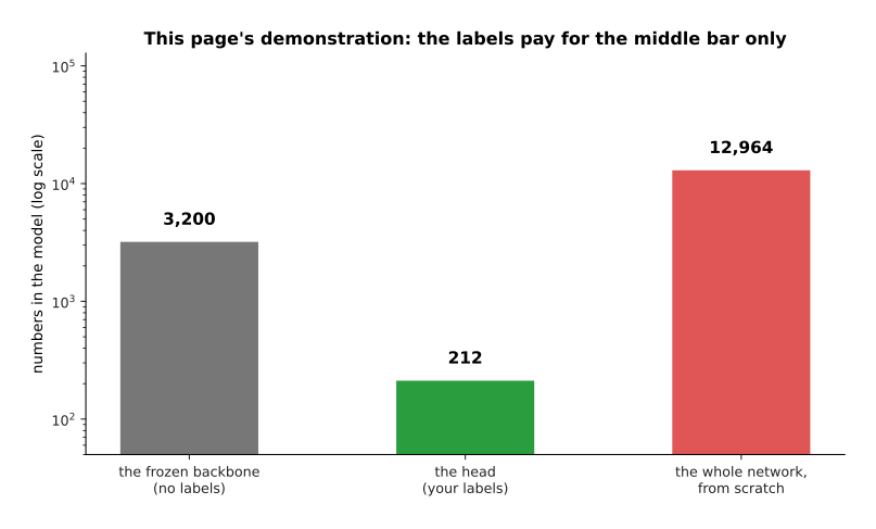
The frozen backbone holds 3,200 numbers and the head holds 212, against 12,964 for a network that learns the same job from scratch on the raw pixels. Your labelled examples only have to fit the 212.
That gap grows much wider at a realistic size. The chart below takes an example backbone of 24 blocks with a width of 1,024 and puts a head for 20 classes on top of it.
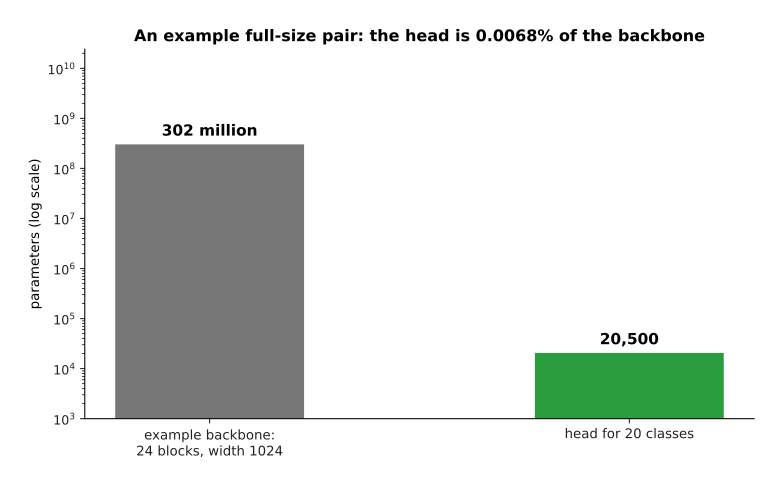
For that example pair the backbone holds 302 million parameters and the head holds 20,500, which is 0.0068 per cent of the backbone.
The backbone used on this page was fitted on 20,000 unlabelled pairs of views. It was fitted by the simplest method of the two-crops kind, one that can be worked out exactly rather than by gradient descent: it keeps the eight directions of the picture on which two views of one item agree most. Six of those directions agree across views with a correlation above 0.91, and the seventh drops to 0.277. That drop is the method finding, without being told, that there are six things worth knowing about these pictures.
The next picture checks what the kept features actually follow. The simulated pictures were built from nine known factors: six that decide what the object is, and three that decide the lighting. Each cell of a grid says how strongly one learned feature follows one known factor, with 1.00 meaning it follows it exactly. The two grids are the same measurement applied to two different ways of choosing features, so compare the left side of each grid with its right side.
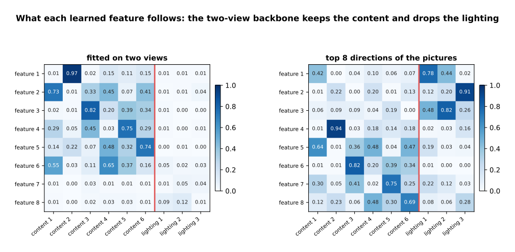
Each feature of the two-view backbone follows a content factor at 0.590 on average and a lighting factor at only 0.037. The eight directions in which the pictures vary most follow a content factor at 0.583 and a lighting factor at 0.422.
That second grid is a warning. Taking the directions of greatest variation also uses unlabelled data, and it fails here, because the lighting varies more than the object does. So what makes a pretext task good is not that it uses unlabelled data. What makes it good is that the thing it forces the model to keep is the thing you will later want.
The chart below puts the three ways of working against each other. It trains a head on top of each representation, and on raw pixels, using training sets of seven different sizes, then measures the accuracy on 4,000 held-out pictures.
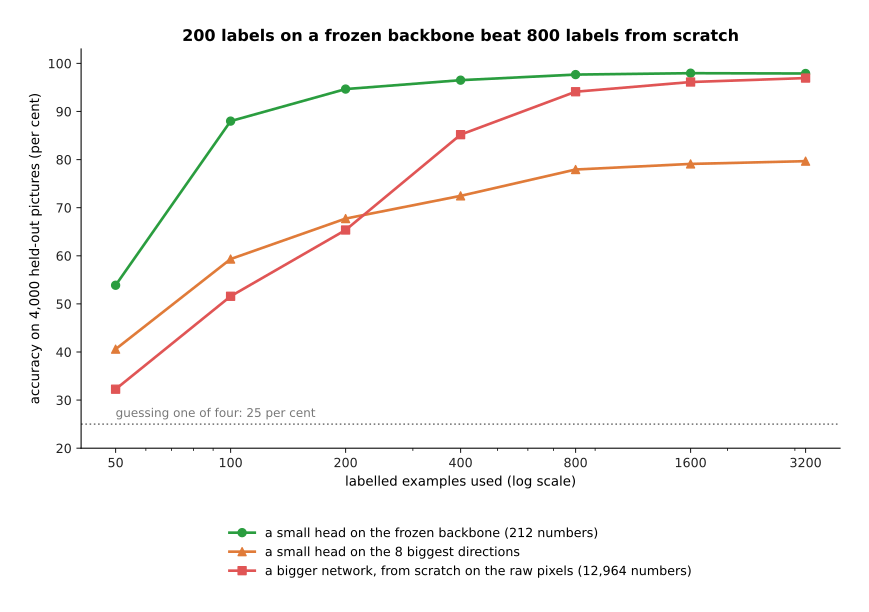
With 200 labels a head on the frozen backbone reaches 94.7 per cent, which the from-scratch network has not reached even with 800 labels, where it reaches 94.1 per cent. The weaker representation never passes 79.7 per cent however many labels it gets.
Read the same result the other way round and the saving is plain. To reach 90 per cent accuracy the head on the frozen backbone needs about 123 labelled examples, while the from-scratch network needs about 581. To reach 95 per cent the numbers are 227 and 1,086. So a few hundred examples on top of a good representation are worth a thousand or more without one, and the backbone itself cost no labels at all. The chart below reads those numbers off the curves for three accuracy targets.
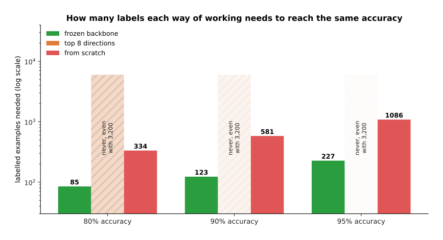
The frozen backbone needs 85, 123 and 227 labels for the three targets, and training from scratch needs 334, 581 and 1,086. The weaker representation reaches none of the three targets.
This is why a large pretrained model is called a foundation model. It is not finished, and it is not useful on its own, but almost everything built afterwards starts from it. What follows is how such a model is made big enough to be worth starting from, which is the next page, and how it is adapted to one job, which is the page after that.
7. Where to read next#
- Scale, data and compute is the next page, and it explains what pretraining actually costs: what a graphics processing unit does, what a parameter costs in memory, and how model size and data size have to grow together.
- Fine-tuning and adapters takes the frozen backbone of section 6 and shows the cheaper ways of adapting it to one job.
- Vision backbones describes the networks that the picture methods on this page are used to pretrain.
- Open-vocabulary vision picks up the promise at the end of section 4 and shows a robot naming an object nobody labelled.
- Large language models follows section 2 to its end, where next-word prediction on a very large amount of text becomes a model that can be talked to.
- Open-vocabulary models is the catalogue page for the real models that this kind of pretraining produced, with what they cost and where they fail.
8. Using it in Python#
Sections 2 to 5 fitted four pretext tasks by hand, so that the arithmetic was visible. This section writes two of those pieces in PyTorch. The first is the contrastive loss of section 4, which is five lines once the vectors exist. The second is the frozen backbone with a head of section 6. The numbers in the comments are the ones this program really prints.
import torch
from torch import nn
from torch.nn import functional as F

torch.manual_seed(0)

# section 4: six pictures and six captions, each already turned into 16 numbers
pictures = F.normalize(torch.randn(6, 16), dim=1)
captions = F.normalize(torch.randn(6, 16), dim=1)

similarity = pictures @ captions.T          # every picture against every caption
match = torch.arange(6)                     # the answer for row i is column i
loss = 0.5 * (F.cross_entropy(similarity / 0.1, match)
              + F.cross_entropy(similarity.T / 0.1, match))
print(round(float(loss), 3))                       # 4.97, before any training
print(round(float(similarity.diagonal().mean()), 3))   # -0.12, the matching pairs

# section 6: a frozen backbone with a small head on top of it
backbone = nn.Sequential(nn.Linear(400, 64), nn.ReLU(), nn.Linear(64, 8))
head = nn.Sequential(nn.Linear(8, 16), nn.ReLU(), nn.Linear(16, 4))
for p in backbone.parameters():
    p.requires_grad = False                 # frozen: gradient descent will not touch it

picture = torch.randn(1, 400)
features = backbone(picture)
print(tuple(features.shape), tuple(head(features).shape))   # (1, 8) (1, 4)
print(sum(p.numel() for p in backbone.parameters()),
      sum(p.numel() for p in head.parameters() if p.requires_grad))   # 26184 212
The first half is the whole of section 4. The grid of similarities is one matrix
multiply. The loss is the ordinary cross-entropy used twice, once down the rows and
once down the columns. The right answer for row i is column i, which is what
the line match = torch.arange(6) says. With untrained vectors the matching pairs
average -0.12, which is no better than any other pair, and the loss is 4.97. The
run in section 4 brought those same two numbers to +0.582 and 1.940.
The second half is section 6. Setting requires_grad to False on every
parameter of the backbone is what "frozen" means in code. The counts printed are
26,184 numbers that pretraining fixed, against 212 numbers that your labelled
examples have to fit. Those two counts are larger than the 3,200 and 212 of
section 6, because this backbone has an extra layer in it.
What a library adds beyond this is the pretrained weights themselves. Hugging
Face's transformers package downloads a backbone that somebody else paid to
pretrain, together with the tokeniser that turns text into exactly the numbers
that model expects, and torchvision does the same for pictures. You almost never
run a pretraining job yourself, because the next page explains what one costs.
What you do decide is which pretrained model to start from, and that is a decision about the pretext task rather than about the architecture. Next-word prediction is good at producing text. Masked prediction is good at understanding a sentence that is already there. The contrastive method of section 4 puts pictures and words in one space. The self-distillation of section 5 gives picture features that ignore lighting and viewpoint. You also decide whether to freeze the backbone at all. Freezing is the cheapest choice and it cannot damage what pretraining learned, but it also cannot repair a backbone that was pretrained on data unlike yours, and robot cameras are often unlike the web.