Running and evaluating a model

The chapter before this one ended with a page on what to do when your model does not work, and the chapter before that finished the book's tour of the model families. Both leave you in the same place. You have a model that has been trained. This page is about what happens next, because a trained model is a file on a disk, and a working robot is something else. The page answers two questions. The first question is what has to happen between that file and an arm that moves. The second question is how you then find out, honestly, whether it works.

The page is for a reader who has followed the book this far, so it assumes you know what weights are, what a loss is, and what a policy gives back. It does not assume you have ever put software into daily use. The things that go wrong here are not the things that go wrong during training, and almost none of them show up as an error message. The page explains each new word where that word first appears. Those words are inference, which means running a trained model rather than training it, runtime, which is the program that carries out the arithmetic, throughput and latency, which are two different ways of being fast, latency budget, success rate, ablation, and out-of-distribution. By the end you will be able to list what a checkpoint must contain, work out whether a model fits inside your control loop, and say how many trials your claim about a robot actually needs.

Every number in the pictures is worked out and printed by docs/diagrams/using_a_model_for_real.py. One example policy runs through the whole page, and one example machine runs it. That machine's speed, its memory bandwidth, and the timings of the camera and of the arm's bus are stated example figures. They are not measurements of any named piece of hardware. The colour-object experiments and the trial experiments use made-up data from a random number generator with a fixed seed, so every run of the script gives the same answer.

Contents#

1. What a trained model is when it is a set of files
2. When the preprocessing does not match the training
3. Export and runtimes: making the file run fast
4. Batching: more answers a second, each one later
5. A latency budget for one arm
6. Judging a model honestly: trials, not loss
7. Reading a failure, and the safety layer that is not learned
8. Where to read next
9. Using it in Python

1. What a trained model is when it is a set of files#

Training ends by writing files to a disk. Those files are the whole of what you have, so it is worth knowing exactly what is in them.

The example policy used through this page works like this. It takes two camera pictures, each 224 pixels high and 224 pixels wide. It also takes a reading of the arm's seven joints and a short instruction written in words. It gives back the next sixteen commands. Inside, its picture encoder is twelve transformer blocks at width 384, and its trunk is six blocks at width 512. A word piece is a short piece of a word, such as gras or ing, and the policy uses a table of 32,000 of them to turn the written instruction into numbers.

The picture below shows the five files that this one trained policy leaves on the disk. The number under each box is how many things that file holds.

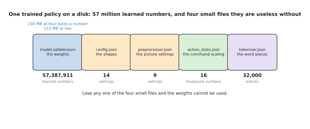
The trained policy is one large file of 57,387,911 learned numbers, together with four small files that say what those numbers mean.

The large file holds the weights. Each weight is stored as four bytes, so the file is 229.6 megabytes. The four small files are the ones people forget, and each of them does a separate job. The configuration file says how many blocks there are and how wide they are, so that the right empty network can be built before the weights are poured into it. The preprocessor file says what size to resize a photo to, what part of it to cut out, and which mean and which spread to subtract and divide by. The command-scaling file holds the smallest and the largest value that each controlled joint took during training. The tokeniser file holds the 32,000 word pieces, so that the same sentence becomes the same numbers it became in training.

It helps to know where the weights actually sit, because people assume the picture encoder holds almost all of them. The chart below gives each part of the policy one bar, and the bar is how many learned numbers that part holds.

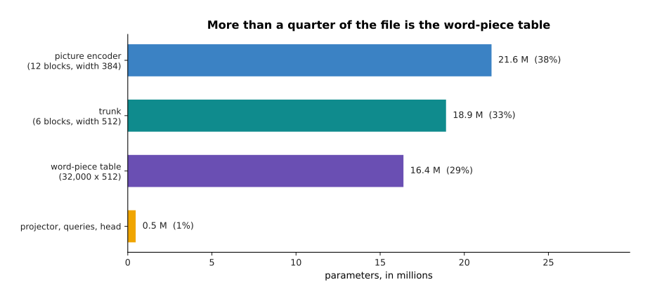
The picture encoder holds 37.7% of the weights, the trunk holds 33.0%, and the table of word pieces holds 28.5%, which is more of the file than most people expect.

That table does no arithmetic at all. It is a lookup table, and it is large because 32,000 word pieces each turned into 512 numbers come to 16,384,000 parameters. So more than a quarter of the file exists only to turn words into numbers.

The size of the file also depends on how many bytes each weight is written with. Writing a weight with fewer bytes stores it less precisely, which the page on making a model smaller and faster explains in full. The chart below shows the same weights written three ways.

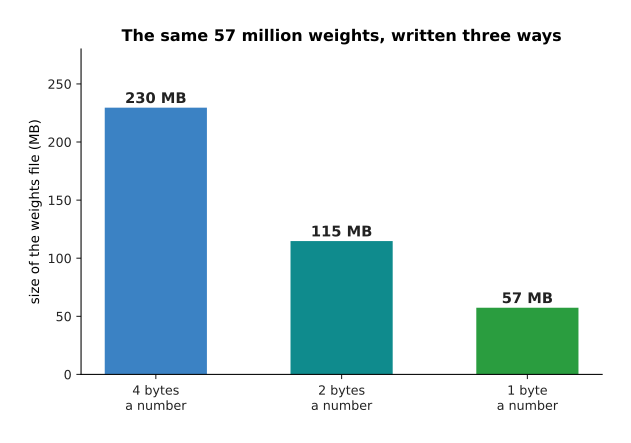
Writing the weights with two bytes a number instead of four halves the file to 114.8 megabytes, and one byte a number brings it to 57.4 megabytes.

That matters when the file has to be copied onto a robot's own small computer, because such a computer often has little storage and little memory. After that, the preprocessor file deserves the same care as the weights, because two sensible settings can give the network two different pictures of one scene.

The four panels below are one scene seen four ways. The first panel is the picture the camera produced. The second and third panels are that same picture prepared in the two ways that real models use. The fourth panel shows, for each pixel, how far apart the two prepared pictures are.

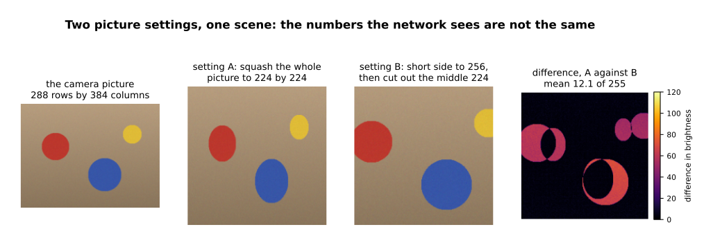
Squashing the whole simulated picture into a square, and cutting a square out of the middle instead, leave numbers that differ by 12.1 out of 255 on average, and 16% of the pixels differ by more than 10.

Neither setting is wrong, and real models use both. What is wrong is to use one of them during training and the other one when the robot runs. The network is then shown a kind of picture it never trained on, and nothing in the system knows that this has happened.

2. When the preprocessing does not match the training#

Section 1 said that the small files decide what the weights mean. This section measures what one wrong small file costs you.

The measurements come from a simulated experiment that the script runs in full. There are four kinds of object, and each kind has its own colour. Each object is photographed under lighting that varies at random. A small classifier is trained on 4,000 of these objects in NumPy, and it is then tested on 2,000 more. With the same settings it trained with, it gets 95.5% of the test objects right.

Preprocessing a picture means subtracting a mean and dividing by a spread, so that the numbers the network sees are centred near zero. If you divide by the wrong spread, nothing breaks and no message is printed. The curve below shows what that costs. The horizontal axis is the spread used when the model runs, written as a multiple of the spread it trained with, so 1.0 means the setting is correct.

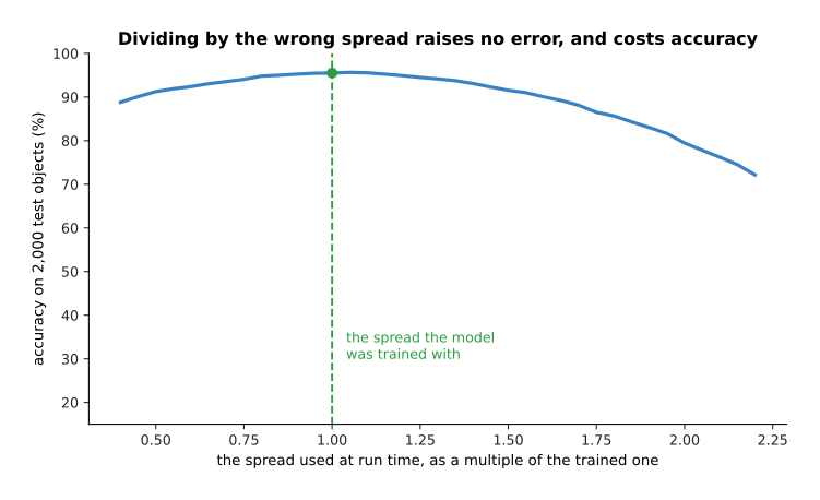
Dividing by twice the right spread drops the classifier from 95.5% to 79.5%, and dividing by half the right spread drops it to 91.2%.

The second setting is the mean that is subtracted. The curve below is the same experiment done on that setting instead. The horizontal axis is how far the mean is out, measured in brightness units that run from 0 to 1.

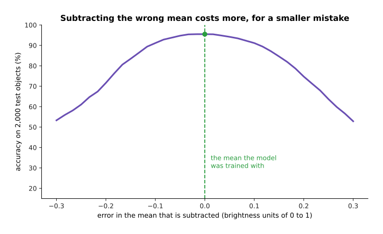
Subtracting a mean that is 0.2 too large drops the classifier from 95.5% to 74.8%, and a mean that is 0.2 too small drops it to 71.7%.

The second curve falls more steeply for a smaller mistake. The reason is that shifting every input by a fixed amount moves the whole cloud of points away from the boundaries the classifier learned, while stretching the cloud leaves its centre where it was. In both cases nothing fails and nothing is written to a log. The model answers every question confidently, and it is simply worse than it was.

The commonest version of this fault is not a wrong number at all. It is a wrong order. A colour picture is three numbers for each pixel, one for red, one for green and one for blue, and those three are called the channels. One popular library hands back a picture with blue first, and another hands it back with red first. The chart below compares the same weights reading the channels in the trained order against the same weights reading them with red and blue swapped.

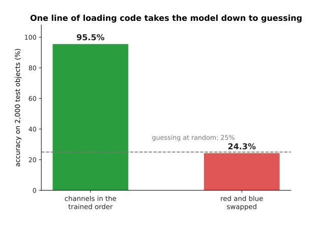
Swapping red and blue takes the same weights from 95.5% down to 24.3%.

With four kinds of object, guessing at random gets about 25% right, so the swap has taken this model down to guessing. The next picture says why this fault is hard to notice. It is a confusion matrix, which means a table whose rows are what the object really was and whose columns are what the model said. Read along a row to see where that kind of object ended up.

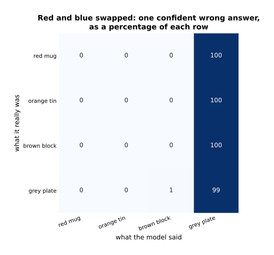
With red and blue swapped, the model calls a red mug, an orange tin and a brown block a grey plate 100% of the time, and it calls a grey plate a grey plate 99% of the time.

So the model is not scattering its answers at random. It is giving one confident wrong answer, over and over. That looks much more like a broken camera than like a broken settings file, which is why people look in the wrong place for it.

The same fault has a second form, and this one is on the output side. A policy gives back numbers between -1 and 1. Those numbers have to be turned back into joint angles, and the command-scaling file does that by stretching the range -1 to 1 onto the range of angles that the training data covered. The chart below draws the lowest and the highest value of each joint, for the right file and for a wrong one that was loaded by mistake.

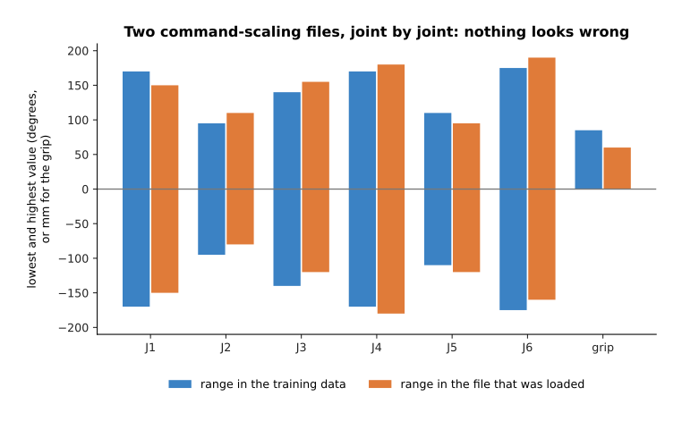
The two files look almost alike, and that is exactly the problem, because nobody checking them by eye would stop on this picture.

The cost of the mistake only appears once the commands are sent. The chart below takes 400 commands from the policy, un-scales each one with the right file and again with the wrong file, and shows how far apart the two answers are, joint by joint.

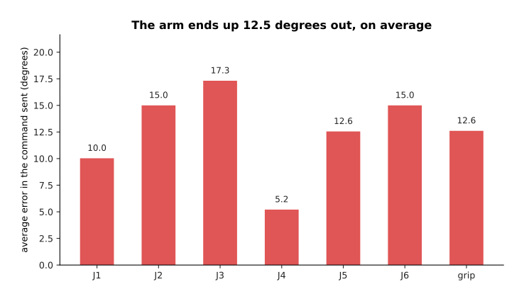
The wrong file sends the arm an average of 12.5 degrees away from where the model meant, and up to 25.0 degrees on a single command.

Joint 3 is the worst at 17.3 degrees. The reason is not that its two ranges differ most in width, because they differ by only 5 degrees. The reason is that the middle of its range moves furthest: the right file runs from -140 to 140 degrees and the wrong one runs from -120 to 155, so the centre shifts by 17.5 degrees and every command inherits that shift. An arm that is 12 degrees out does not look like a software fault. It looks like a badly trained policy, and people then spend weeks collecting more data to fix a one-line mistake. The habit that prevents all of this is to save the preprocessing settings inside the checkpoint, beside the weights, and never to retype them anywhere else.

3. Export and runtimes: making the file run fast#

Section 2 got the right numbers into the model. This section gets the answer out of it quickly.

Running a trained model is called inference, and the word exists to separate it from training. The obvious way to do inference is to call the same training framework that made the model. That works, and it is slow, for reasons that have nothing to do with the arithmetic.

Start with the arithmetic itself, because that is the floor that nothing can go below. The unit here is the multiply-add, which is one multiplication followed by one addition, and it is the operation a neural network spends nearly all of its time on. The chart below counts the multiply-adds in one decision and splits them by which part of the policy does them. The scale is logarithmic, so each step along the axis is ten times the one before.

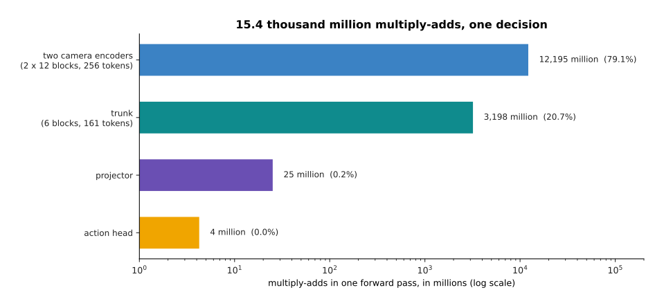
One decision costs 15.4 thousand million multiply-adds, and 79.1% of them belong to the two camera encoders.

The example machine is stated to get through 1.2 million million multiply-adds a second when numbers are four bytes, 3.6 million million when they are two bytes, and 7.2 million million when they are one byte. It is also stated to move 100 thousand million bytes a second to and from its memory. Those two abilities compete, because the machine has to read every weight out of memory before it can use it. The chart below compares the time the arithmetic needs with the time that reading the weights needs, at all three precisions.

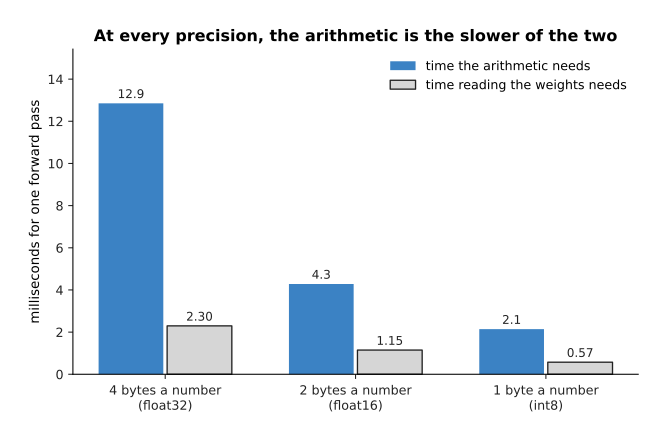
At four bytes a number the arithmetic takes 12.85 milliseconds and reading the weights takes 2.30, so the arithmetic is the slower of the two, and it stays the slower one at every precision.

A model whose arithmetic is slower than its memory reading is said to be limited by arithmetic, and this one is. So 12.85 milliseconds is the floor at four bytes a number. The training framework does not reach that floor, because it hands the graphics processor one small piece of work at a time and then waits for the answer before sending the next one.

Each of those hand-offs costs time whether the piece of work is large or small. The chart below counts the pieces of work in one decision, first as the training framework runs them, and then after they have been joined together.

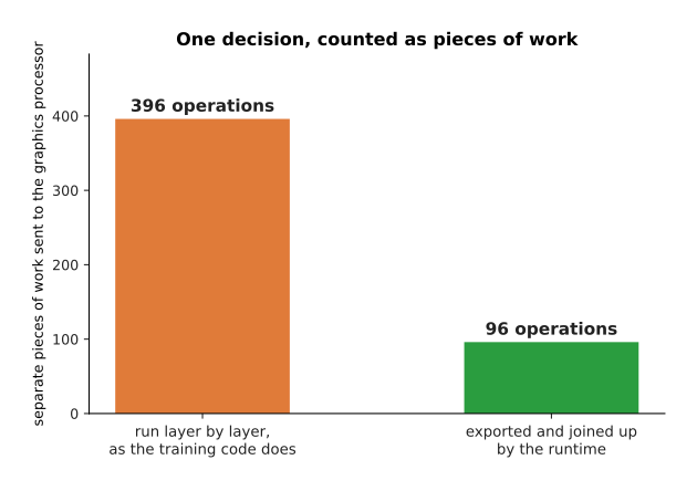
Joining the operations up turns 396 hand-offs into 96.

Exporting a model means writing it out as a fixed graph of operations, with no Python left inside the loop. A runtime is the program that then carries that graph out. The runtime sees the whole graph at once, so it can join a normalisation, a matrix multiply and an activation into a single piece of work, and that is how 396 becomes 96. The chart below turns that saving into milliseconds, at the example cost of five microseconds for each hand-off.

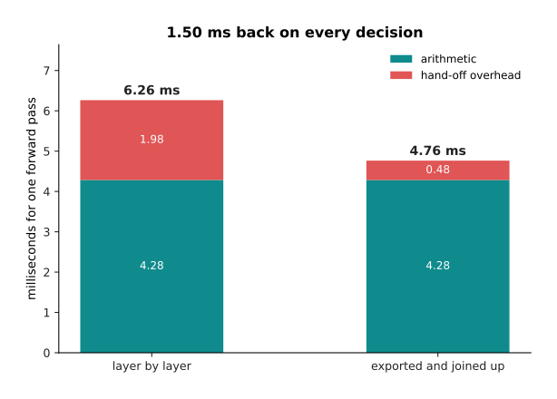
Removing 300 hand-offs at five microseconds each gives 1.50 milliseconds back, which is 24% of the time the layer-by-layer version took.

Export is not one change, it is several, and they do not all buy the same thing. The picture below lists them in the order you would apply them, with the time one forward pass takes after each step.

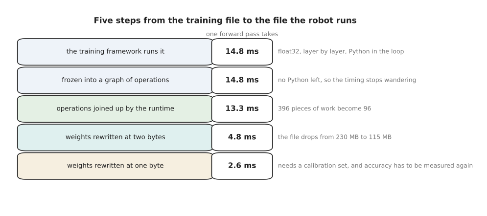
The same model goes from 14.8 milliseconds to 2.6 milliseconds in five steps, and each step costs you something different.

Freezing the graph buys steadiness rather than speed, because the time one call takes stops wandering with whatever else Python happened to be doing. Rewriting the weights with two bytes a number is the large win, at 4.8 milliseconds, and one byte a number gets to 2.6. However, that last step needs a calibration set, which is a small batch of real inputs used to choose the scale of the smaller numbers, and the accuracy has to be measured again afterwards, as making a model smaller and faster explains. The reason to export rather than to keep calling the training framework is those numbers. The cost is that the exported file is harder to look inside, and it has to be built again every time the model changes.

4. Batching: more answers a second, each one later#

Section 3 made one forward pass fast. The obvious next idea is to do several forward passes at once.

Working out several answers in one call is called batching, and it is the first thing anybody suggests when a model is too slow. It works because each call pays a fixed cost once, however many items are in it. Here that fixed cost is 0.48 milliseconds of hand-offs, 1.15 milliseconds of reading the weights out of memory, and a stated 1.2 milliseconds of waking the machine up and waiting for it to answer, which comes to 2.83 milliseconds. Each item in the batch then pays 4.36 milliseconds of its own arithmetic and copying.

The two panels below are the same batching experiment measured two ways. The left panel counts answers a second. The right panel counts milliseconds, both for the whole call and for one decision's share of it.

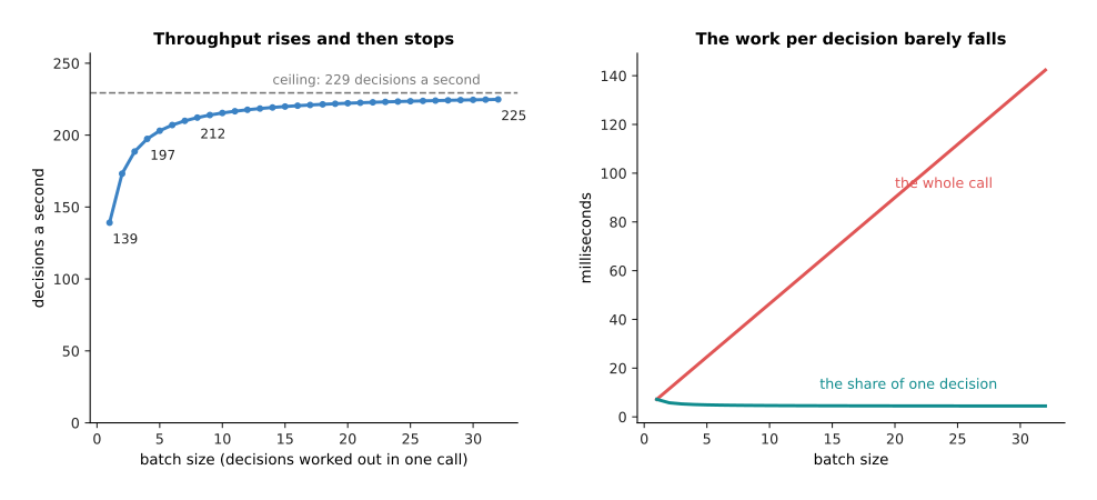
Throughput, which means answers a second, rises from 139 at a batch of one to 212 at a batch of eight, and then creeps towards a ceiling of 229.

Most of the gain has arrived by a batch of four, which gives 197 a second. The reason is that all batching can do is spread one fixed cost over more items, and that fixed cost is only 2.83 milliseconds of the 7.19 milliseconds a single call takes. A batch of 32 gives 1.62 times the throughput of a batch of one, so batching is a modest win for a model whose cost is mostly its own arithmetic.

The cost of that win falls on latency, which means the time from one picture arriving to the command for that same picture going out. Latency gets worse because an arm cannot be given an answer until the batch it is sitting in has been filled, and filling it means waiting for other arms to ask. The chart below shows the worst time from picture to command, for four different numbers of arms sharing one machine.

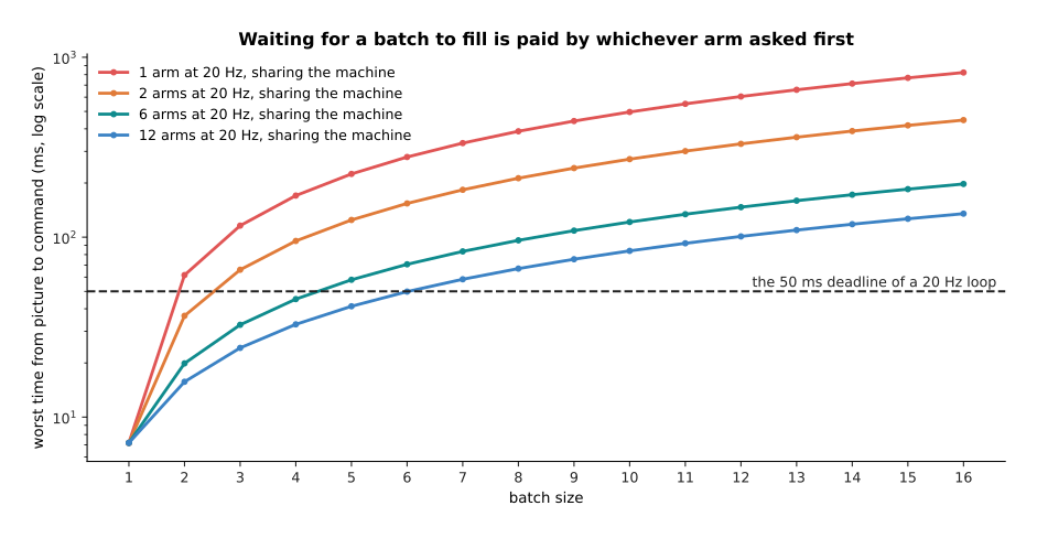
With one arm asking twenty times a second, no batch larger than one meets the 50 millisecond deadline, and it takes twelve arms sharing the machine before a batch of six does.

Every extra place in the batch adds one more arrival interval of waiting for whoever asked first. The timeline below follows that unhappy case all the way through, for two arms sharing a batch of eight.

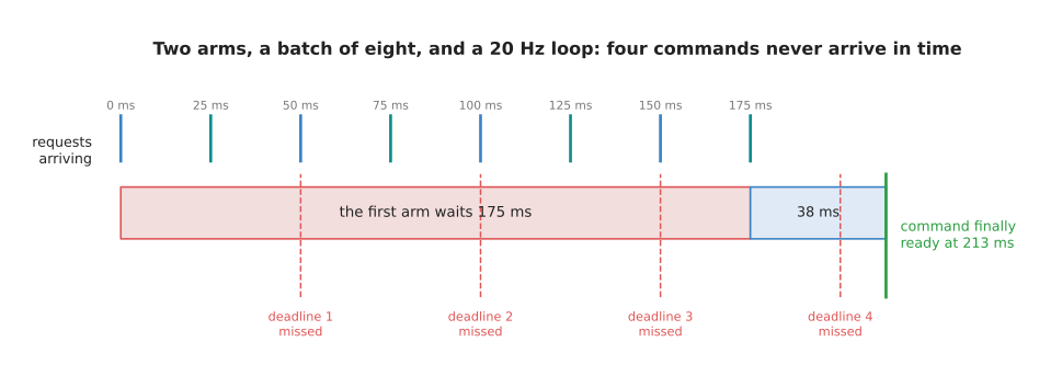
The first arm waits 175 milliseconds for the batch to fill, and its command is ready 213 milliseconds after its own picture arrived, by which time four 50 millisecond deadlines have passed.

So batching is right in two situations. It is right when many arms share one machine, and it is right when you are scoring a recorded dataset and nobody is waiting for the answer. It is wrong for one arm inside a control loop.

5. A latency budget for one arm#

Section 4 measured the model's own time. This section puts that time next to everything else in the loop, because the model is never the only thing in it.

A latency budget is a written list of every stage between the light reaching the camera sensor and the command reaching the arm, added up and compared with the period of the control loop. The period is how long one turn of the loop is allowed to take. The example here runs at 20 hertz, which means twenty turns a second, so the period is 50 milliseconds. Every stage time below is a stated example except the forward pass, which is section 3's measured 4.76 milliseconds.

The bar below is the whole budget, drawn end to end. Each coloured block is one stage, and the dashed lines mark the periods of three different control rates.

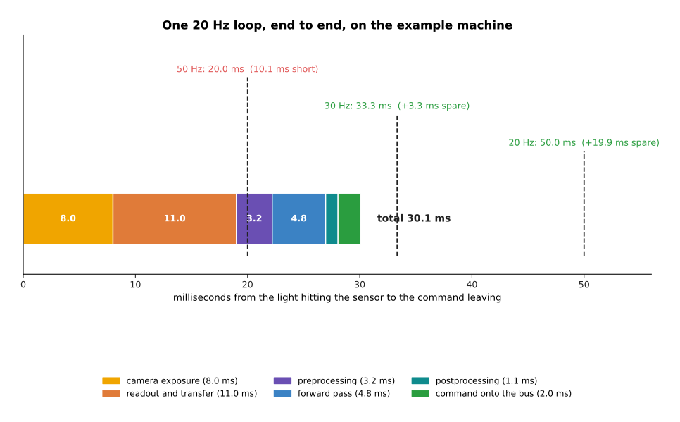
The whole loop takes 30.1 milliseconds, which leaves 19.9 milliseconds spare at 20 hertz and 3.3 milliseconds spare at 30 hertz, and which falls 10.1 milliseconds short at 50 hertz.

The stages are these. The camera exposes for 8.0 milliseconds. It then reads the picture out and sends it over the cable, which takes 11.0 more. The preprocessing of section 1 takes 3.2 milliseconds. The network takes 4.76. Turning the network's output back into joint angles takes 1.1. Putting the command on the arm's bus takes 2.0. The budget does not fit at 50 hertz, and that is a fact about the camera rather than about the network.

The two panels below are the same 30.1 milliseconds grouped two ways. The left panel gives each stage its own bar. The right panel puts the two camera stages together and everything else together.

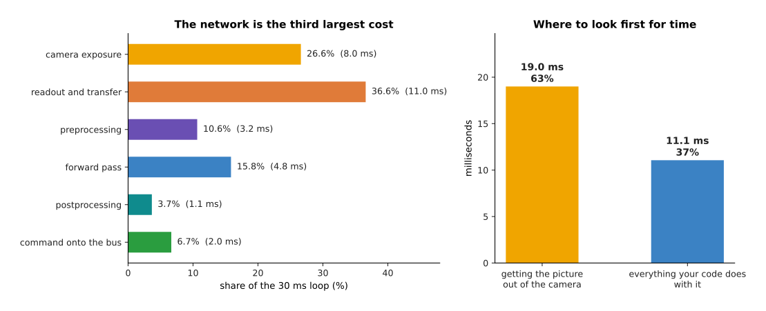
Getting the picture out of the camera takes 19.0 milliseconds, which is 63.2% of the loop, while the network takes 15.8% of it.

The network is only the third largest cost, behind the camera's readout and its exposure. So shaving a millisecond off the network is hard work for a small return, while buying a faster camera is usually worth more. Exposing the next picture while the current one is still being processed is worth more again, and it costs nothing but code.

There is one more way to buy time, and it comes from the policies of diffusion and flow policies, which give back a whole chunk of future commands rather than one command. The timeline below shows three such chunks, each one started before the last one ran out.

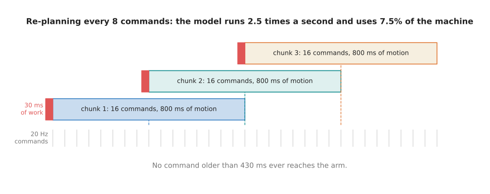
A chunk of sixteen commands covers 800 milliseconds of motion, so re-planning after every eight commands means the model runs 2.5 times a second and uses 7.5% of the machine.

The arm still receives a command every 50 milliseconds. However, those commands now come out of a list that the model wrote earlier, so the model's own deadline is 400 milliseconds rather than 50. What this costs is freshness. The last command of each half-chunk was worked out from a picture taken up to 430 milliseconds before it is used, which is far too old if something in the scene is moving. So the question to ask is not how fast the arm can be commanded. The question is how fast the world changes.

6. Judging a model honestly: trials, not loss#

Sections 1 to 5 got the model running. This section asks whether it works.

The number that training gives you is a loss on a held-out set, which means a score on examples the model never trained on. It is tempting to treat a lower loss as a better robot, but those two things are only loosely tied together. The script shows this with 180 simulated policies. Each policy makes a small position mistake at every step of a 40-step reach. The arm carries part of its error forward from one step to the next, and the grasp succeeds only if the error never leaves an 11 millimetre tolerance. Some policies also make a rare large mistake. Each dot below is one of those 180 policies, and the colour says how often that policy makes a large mistake.

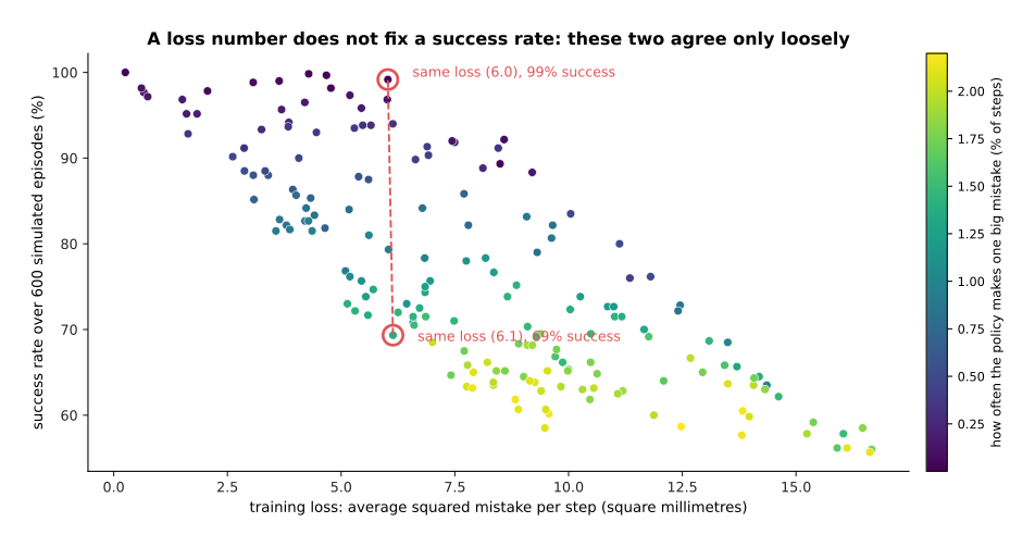
Loss and success rate agree only loosely, and two of the simulated policies, with losses of 6.1 and 6.0 square millimetres, succeed 69% and 99% of the time.

The reason is in the colour. A policy whose mistakes are small and steady keeps the arm inside the tolerance even when its average squared error is large. A policy that throws one large mistake every seventy steps fails whenever that mistake happens to land during a grasp. The loss averages over steps, and the task does not average over anything, because one bad step ruins the whole attempt. So the only honest measure of a robot policy is a success rate, which means the fraction of whole attempts that worked.

That rate is only honest if the attempts were chosen before you saw any results. An evaluation protocol is a list, written in advance, of how many trials you will run, where the object starts in each one, and what counts as a success. The heat map below is that list drawn out. The workspace is divided into 48 cells, twelve trials are run in each cell, and the number in each cell is the share of those twelve that succeeded. The dots are where the demonstrations put the object during training, and the dashed box encloses them.

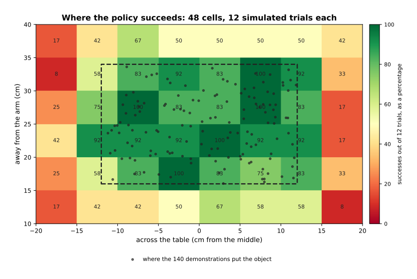
The policy succeeds almost everywhere inside the dashed box, and it falls away quickly outside it.

The chart below adds those cells up on each side of the dashed box, so the two scores can be compared directly. The black bars show the 95% confidence interval, which the next picture explains.

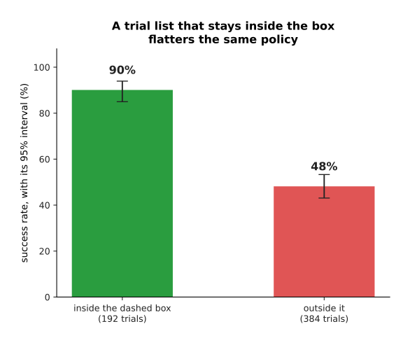
In this simulation the same policy scores 90% in the 192 trials inside the box the demonstrations covered, and 48% in the 384 trials outside it.

Inputs that the model was not trained on are called out-of-distribution, which means they come from a different mix of situations than the training data did. A trial list that stays inside the green middle reports 90%, and that number is not a lie about anything except what the robot will do tomorrow. The second thing the trial list decides is how many trials to run, and this is where most reported numbers fall apart.

A 95% confidence interval is a range built so that, if you repeated the whole experiment many times, the range would contain the true rate 95 times in 100. The chart below draws that range for two scores, 70% and 90%, measured with six different numbers of trials.

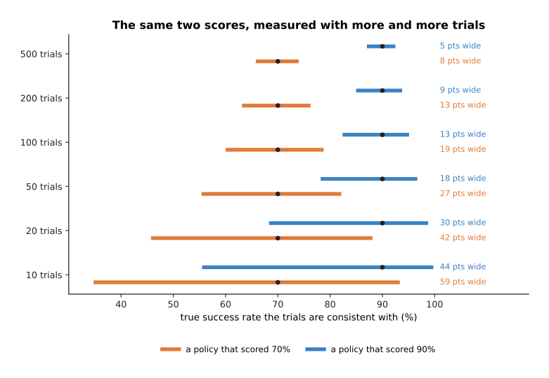
Eighteen successes in twenty trials is consistent with a true rate anywhere from 68.3% to 98.8%, so that interval is 30.5 percentage points wide, and the interval for a score of 70% at twenty trials is 42.4 points wide.

Those two intervals overlap heavily, so twenty trials cannot tell the two policies apart. The chart below puts an exact number on that. It takes two policies that really are 70% and 90%, runs the same number of trials on each, and asks how often the two intervals come out separated.

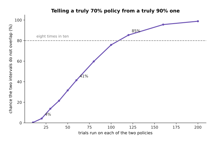
Twenty trials each tell a truly 70% policy from a truly 90% one only 4 times in 100, and it takes about 120 trials each before that happens 85 times in 100.

So a table of twenty-trial numbers is a table of noise. The same arithmetic governs ablations, which means taking one part of the system away and measuring what happens, in order to find out which parts matter. The chart below runs four versions of the same policy, 80 simulated trials each, and writes each version's training loss inside its bar.

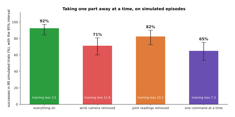
With 80 simulated trials each, the last three versions score 71%, 82% and 65%, their intervals all overlap, and their training losses of 11.8, 10.2 and 7.3 put them in a different order again.

Each bar is a separate simulation in which exactly one thing changes. Removing the wrist camera makes every step noisier. Removing the joint readings adds a steady lean to one side. Giving one command at a time, instead of a chunk, makes consecutive mistakes repeat. The full system at 92% beats all three. However, the three cannot be put in order against each other at 80 trials, and the loss ranks them differently again, so neither number on its own would have told you which part to keep.

The last thing to be careful about is a benchmark number. A benchmark tells you how a model did on somebody else's objects, lighting and arm. That helps you choose what to try, and it says nothing about your own cell. The chart below measures the shape of that gap, using the colour classifier from section 2 under four conditions.

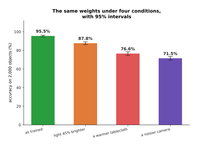
The same weights score 95.5% on the conditions they trained on, 87.8% under light that is 45% brighter, 76.6% against a warmer tablecloth and 71.5% through a noisier camera.

None of those four changes is dramatic, and none of them is anything a person would mention, which is the point. The curve below sweeps the brightness continuously instead of testing four fixed conditions, so you can see the whole shape of the fall.

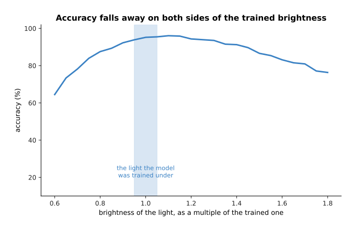
Accuracy falls away on both sides of the brightness the model trained under, reaching 64% when the light is 0.6 times as bright and 76% when it is 1.8 times as bright.

On a real arm the list of such changes includes a sunnier afternoon, a new tablecloth, and a replacement gripper whose fingers are three millimetres narrower, so that every grasp closes slightly too early. Any one of them means running the evaluation again, because nothing in the training promised anything about them.

7. Reading a failure, and the safety layer that is not learned#

Section 6 counted failures. This section is about understanding a single one of them.

When an arm knocks a mug over, three different things can have happened, and from outside the robot they look the same. The perception may have lost the object. The policy may have chosen badly while seeing the scene perfectly well. The hardware may have refused to do what it was told. Telling them apart means reading three recorded streams against each other, so the next three pictures are three simulated episodes, one for each kind of failure.

The first episode is a perception failure. The detector score is how sure the detector is that it has found the object, and the target is the position the policy was handed.

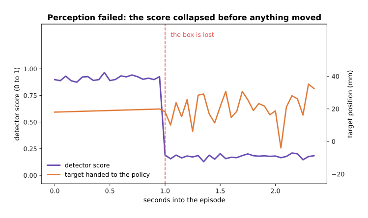
The detector score collapses first, and only after that does the target start jumping about, by up to 25 millimetres from one step to the next.

The second episode is a policy failure. Here the detector keeps working, and the command itself goes wrong, so the picture draws the command against the smooth answer a steady policy would have sent.

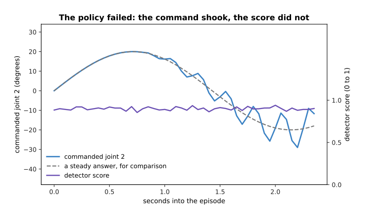
The command shakes at 4 hertz and grows to 9.8 degrees away from the smooth answer, while the detector score stays at 0.90 and never moves by more than 0.07.

The third episode is a hardware failure. Here the command is smooth and correct, and the joint does not follow it.

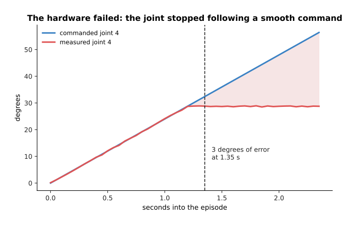
The measured joint stops at 28.8 degrees while the command keeps rising to 56.4, so the tracking error passes 3 degrees at 1.35 seconds.

Read those three pictures as a procedure. Look at the perception output first, because if the detector score fell before anything else moved then the policy was acting on nonsense. If perception held steady, compare the command with what a steady policy would send, because a command that oscillates at a few hertz is a policy flipping between two answers. If the command is smooth, compare it with the measured joint position, because a gap that grows is a motor, a cable or a collision, and no amount of retraining will help with any of those.

That procedure only works if the streams were recorded, and recording everything is not free. The two panels below are the same list of streams counted two ways. The left panel gives each stream its own bar, on a logarithmic scale because they differ enormously. The right panel adds them up.

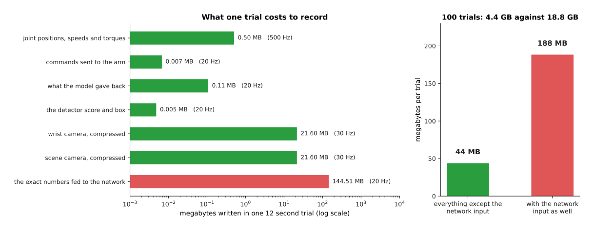
A twelve-second trial costs 43.8 megabytes when you keep the two compressed camera streams, the joint readings at 500 hertz and the model's own output, so 100 trials come to 4.4 gigabytes.

The joint readings cost half a megabyte a trial, and the two compressed camera streams cost 21.6 megabytes each. The exact block of numbers fed into the network costs 144.5 megabytes on its own, which is more than three times everything else put together, so keep that one only for trials that failed. The page on sensor streams describes how such streams are recorded with their timestamps lined up, which matters here because a log whose timestamps are not lined up cannot say which thing happened first.

The last thing to say about failure is that the model must not be the only thing protecting the arm, because a trained network comes with no guarantee at all. Nothing in the training says that its output will stay inside the joint limits. Nothing says that it will not ask for an impossible speed. Nothing says that it will answer at all.

So a layer of ordinary written code sits between the model and the motors, and that layer is not learned. Its first job is to clamp every command, which means refusing to pass on anything outside the joint limits and anything that moves further in one period than the speed limit allows. The chart below shows that clamp working on simulated commands.

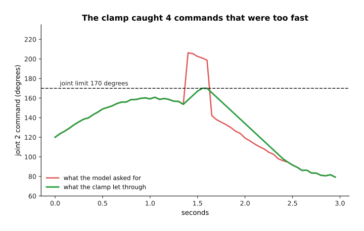
The clamp caught 4 of the 59 command changes, and it held the peak speed at the 90 degrees a second limit instead of the 1,132 degrees a second the policy asked for.

The clamp's second job is to notice when no command arrives at all. A watchdog is a timer that is reset by every command and that stops the arm if it ever runs out. The timeline below shows one.

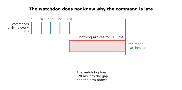
The watchdog brakes the arm 120 milliseconds into a 300 millisecond silence, which is 2.4 command periods, and it does that without knowing why the commands stopped.

So the written layer clamps every command to the joint limits, it limits how far a command may move in one period, which at 20 hertz and 90 degrees a second is 4.5 degrees, it stops the arm when the measured force passes a threshold, and it brakes the arm if no command arrives within 120 milliseconds. The reason to write this layer rather than to train it is that written code can be read, argued about and tested exhaustively, while a network cannot. The cost is that the clamp sometimes spoils a legitimate fast motion. The safety monitoring page describes how such a layer is built, and proportional-integral-derivative (PID) control describes the controller that sits underneath it.

8. Where to read next#

• The map of models is the next page and the last of this book, and it maps every family the book explained, with a table of what to reach for.
• Diffusion and flow policies explains the action chunks and the control frequencies that section 5's budget depends on.
• Making a model smaller and faster explains quantisation and distillation, which are the two largest levers in section 3's list of steps.
• Overfitting and generalisation explains the split that section 6's loss number comes from.
• Running a model on a robot is the catalogue page for this subject, written about real named models.
• Evaluation and failure is the catalogue page for section 6, with a worked mug-picking evaluation.

9. Using it in Python#

Section 1 said that a checkpoint is weights plus settings. Section 3 timed a forward pass. Section 6 turned a count of successes into a range. The code below does all three, with a model small enough to run on any computer.

import time
import numpy as np
import torch
from torch import nn

# Section 1. Save the settings with the weights, so the two cannot drift apart.
policy = nn.Sequential(nn.Linear(14, 64), nn.ReLU(), nn.Linear(64, 7))
settings = {
    "image_size": 224, "crop": "centre",                      # the preprocessor file
    "pixel_mean": [0.485, 0.456, 0.406], "pixel_std": [0.229, 0.224, 0.225],
    "channel_order": "RGB",                                   # section 2's commonest fault
    "action_low": [-170.0] * 7, "action_high": [170.0] * 7,   # the command scaling
}
torch.save({"weights": policy.state_dict(), "settings": settings}, "policy.pt")
print(sum(p.numel() for p in policy.parameters()))            # 1415

# Section 3. Freeze the graph, then time one forward pass properly: warm up first.
policy.eval()
example = torch.zeros(1, 14)
frozen = torch.jit.trace(policy, example)
with torch.inference_mode():
    for _ in range(50):
        frozen(example)
    start = time.perf_counter()
    for _ in range(500):
        frozen(example)
print(f"{(time.perf_counter() - start) / 500 * 1000:.3f} ms per call")

# Section 2. Un-scale with the settings that were saved, never with retyped ones.
low = np.array(settings["action_low"])
high = np.array(settings["action_high"])
with torch.inference_mode():
    raw = frozen(example).numpy()[0]                          # the -1 to 1 output
print(np.round(low + (raw + 1) * 0.5 * (high - low), 1))      # joint angles in degrees

# Section 6. The exact 95% interval for 18 successes in 20 trials.
from scipy.stats import beta
successes, trials = 18, 20
lo = beta.ppf(0.025, successes, trials - successes + 1)
hi = beta.ppf(0.975, successes + 1, trials - successes)
print(f"{100 * successes / trials:.0f}%  from {100 * lo:.1f}% to {100 * hi:.1f}%")
# 90%  from 68.3% to 98.8%

The parameter count of 1,415 is 14 times 64, plus 64 biases, plus 64 times 7, plus 7 biases. The interval of 68.3% to 98.8% is the one section 6's picture draws for eighteen successes in twenty trials, and scipy works it out from the beta distribution in two lines. The timing line prints whatever your own machine gives, and that is the one number on this page that nobody can work out for you.

The libraries do a lot of this work for you. torch.jit.trace and the newer torch.compile freeze the graph of section 3. ONNX Runtime and TensorRT are runtimes that then join the operations up, where ONNX is the Open Neural Network Exchange format that holds the frozen graph. The transformers and timm packages ship preprocessing settings beside their weights, which makes section 2's fault harder to make in the first place.

What you still have to decide is everything the libraries have no view on. You choose the control rate, and therefore the budget that every stage in section 5 must fit inside. You choose what to log and what to throw away. You write the trial list of section 6 before you run it, knowing now that twenty trials distinguish almost nothing. And you write the safety layer of section 7 yourself, because it is the one part of the system that must still work when the model is wrong.