This page judges this solution. It says where the solution is strong and where it breaks. It names the general ideas behind it. Then it places it beside the other five.
Contents#
- Where it is strong and where it breaks
- The general ideas behind this
- Where it sits among the other five
1. Where it is strong and where it breaks#
The earlier pages showed how the solution works. This section shows how well.
The examiner scored it on five blocks of 20 held-out arrangements. The table below gives its score row. Read each row as one kind of arrangement. "Found" is glasses found out of every 100. "Place error" is the median distance from the true place.
| Arrangements | Found per 100 | Place error (median) |
|---|---|---|
| Spaced by the cell's layout rule | 64.1 | 0.6 mm |
| Crowded closer than the rule allows | 74.6 | 0.9 mm |
It does better on the crowded set. Every other solution does worse there. The end of this section explains why.
It has no domain gap. All it knows came from this cell's own pictures. What it is explains why that makes it the control.
It separates glasses that are joined in the picture. Nothing has to find a boundary, so no boundary can be wrong.
It is good at a partly hidden glass. A thin crescent of a glass still votes for the right middle. The worked example shows this.
Its doubt is a measurement. The number of votes in a pile says how sure to be. It is measured from the votes, not guessed by the network.
It cannot see a fully hidden glass. No pixels means no votes. This is true of every method that reads pictures.
It cannot see a glass whose own middle is outside the picture. This is its biggest loss by far. Votes are counted in a tally the size of the picture. A vote that lands outside it is dropped. Splay pushes a tall glass's middle outwards. If the glass stands near the side of the glass zone, its middle can land past the edge of the picture. Then all its votes are dropped, and no pile forms.
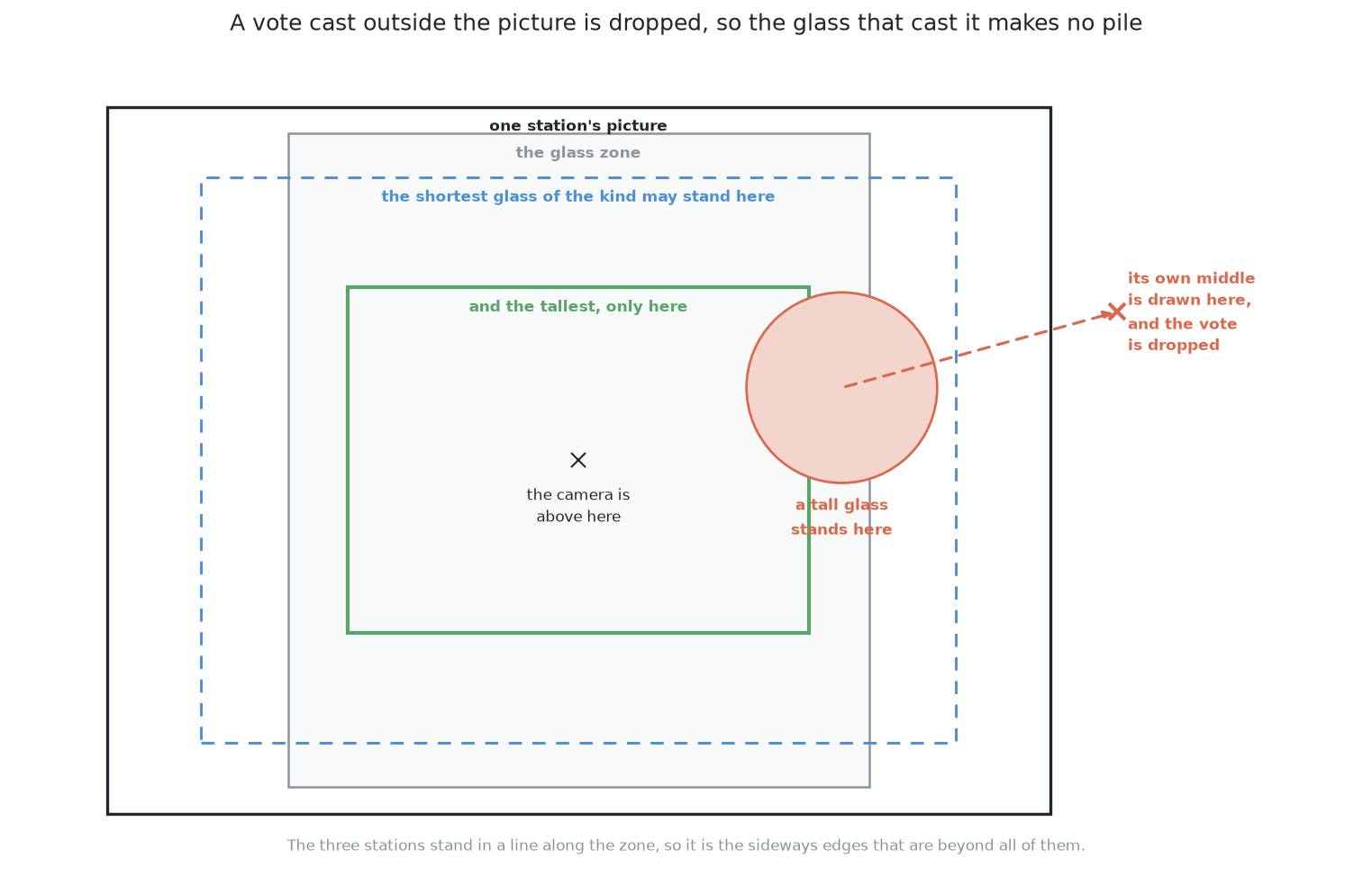
This loss can be counted without running the network. In the spaced arrangements, 499 glasses were seen by some station. Only 312 of them, 62.5 per 100, had their middle inside the picture at any station. The solution found 64.1 per 100. So it already finds about as many glasses as this limit allows. The problem is the voting design, not the training. In the crowded arrangements, the same count is 87.0 per 100. This is because the crowded arrangements put their glasses in lines under the middle station. There the solution found 74.6. This is why it does better on the crowded set.
So the fix is not more training. The fix is a tally bigger than the picture. Then a middle past the edge still has a place to land.
It needs a training set and a training run first. A downloaded model can answer on the first day. This one cannot.
It cannot explain its answer. When a written rule is wrong, you can print a number and see why. When a network is wrong, you can only guess. The width check after the network helps here.
Its weights must match the cell. What it needs explains this cost.
These strengths and weaknesses come from a few general ideas. The next section names them.
2. The general ideas behind this#
The last section judged this solution. This section names the standard ideas it is built from, so you can find them elsewhere. Most of them are not new. Two things are unusual here. The network is trained from random numbers, not fine-tuned. And one network answers both "is this glass?" and "which glass?".
Semantic segmentation — a class label at every pixel#
Semantic segmentation gives a label to every pixel, not a box round an object. Fully convolutional networks made it practical (Long, Shelhamer and Darrell, arXiv:1411.4038).
It is used where the shape of a thing matters, such as medical images, aerial pictures and factory inspection. It is not right for counting or separating objects. A class label cannot say which object a pixel belongs to. The second head here exists to fix that. For more, see image segmentation.
The encoder–decoder with skip connections#
This is the U-Net described in the shape of the network (Ronneberger, Fischer and Brox, arXiv:1505.04597). It was made for medical images with very few training examples. So it suits a small training set.
It is still the usual choice for a small segmentation problem. It is not right when a problem needs broad knowledge of scenes or many classes. A small network knows only what it saw in training.
Overlap losses — scoring the shape rather than the pixel count#
Dice and intersection over union losses score the overlap between the answer and the truth. The first head explains why they help (Milletari and colleagues, arXiv:1606.04797).
They are used wherever one class is much rarer than the other. This covers most medical and factory segmentation. They are rarely enough alone. They do not say how sure each pixel was, and a feedback loop can use that.
The Hough transform — local evidence for a global claim#
One edge pixel cannot say where a shape is. But it can vote for every shape that would explain it. Add up the votes, and the peaks are the real shapes. Hough's 1962 patent did this for straight lines. The generalised Hough transform (Ballard, 1981) did it for any shape, using a table of offsets.
It is used to find shapes in cluttered pictures where much of the outline is missing. The visible part still votes correctly. It is not right for shapes with many settings, because the table of votes grows too large. For more, see the Hough transform.
Learned voting — replacing the table of offsets with a model#
Hough forests (Gall and Lempitsky, 2009) first learned the table of offsets instead of building it by hand. Later networks do the same. VoteNet (arXiv:1904.09664) has depth points vote for object middles. PVNet (arXiv:1812.11788) has pixels vote for key points, because voting still works when part of an object is hidden.
These are used for cluttered scenes and bin picking. They are not right for objects with no clear middle. They also struggle when the arrows are long compared with the picture, because the votes then scatter.
Mean shift — finding peaks without being told how many#
From votes to glasses describes mean shift (Comaniciu and Meer, 2002). It does not need the number of groups in advance. That is the point here, because the number of groups is the answer.
It is used for tracking and colour segmentation. It is not right for data with many dimensions, where it is slow and the window size is hard to choose. It is also poor when groups have very different densities. For more, see mean shift.
Self-supervised learning — labels from the structure of the data#
Self-supervised learning makes up a task whose answer is already in the data. So labels are free. The second way does this with the arm's encoders.
It is used where data is plentiful and labels are costly. It suits robotics, because a robot always knows its own position. It fails when the task has a shortcut that skips the skill you wanted. Designing a task with no shortcut is the hard part. For more, see self-supervised learning.
Geometry as supervision, and depth without depth labels#
Suppose you know how the camera moved between two pictures. Then a point's place in the first picture and its depth say where it must be in the second. This is the epipolar constraint. It turns a depth guess into a prediction you can check. SfMLearner (Zhou and colleagues, arXiv:1704.07813) trained depth this way with no depth labels. Monodepth2 (Godard and colleagues, arXiv:1806.01260) fixed most of its problems.
Those methods must estimate the camera's movement, and much of their error comes from that. In this cell, the movement is known exactly. The approach is not right for surfaces with no texture. It also fails when objects move between the two pictures. For more, see structure from motion.
Grouping by shared motion — common fate#
Points on one surface move together in the picture. Points on a surface at a different distance do not. Gestalt psychologists called this common fate. It needs no knowledge of how things look. So it works on two identical glasses.
It is used for video segmentation and tracking. It is not right when nothing moves relative to anything else. This is why the second way is weak from above. Two rims at the same height barely move relative to each other.
Contrastive training — turning "these belong together" into a loss#
What contrastive training does describes the method. The standard references are SimCLR (Chen and colleagues, arXiv:2002.05709) and MoCo (He and colleagues, arXiv:1911.05722). A related idea gives each pixel an identity code and groups the codes. It is called associative embedding (Newell and colleagues, arXiv:1611.05424).
It is used where pairs that belong together are easy to make, but categories are not. It is rarely enough alone when the count matters. An embedding never says how many groups there are. The checks after the network fill that gap here.
Training from scratch against fine-tuning a large model#
This is the choice the whole chapter rests on. Fine-tuning wins when labels are scarce, which is almost always. Training from scratch wins only when labels are free, the problem is small, and borrowed weights know a different world. This cell is that rare case. Do not take it as a general rule.
The next section places this solution beside the other five.
3. Where it sits among the other five#
The general ideas show what this solution is made of. This section says what its place in the comparison tells you.
This solution borrows nothing, so it is the control. The four learned solutions that borrow weights all have a domain gap. This one has none. So the difference between this solution and those four measures what borrowing was worth. The rules on the table solution is the written-rule baseline. Comparing with it asks whether a trained grouping beats a written one.
The six solutions side by side makes these comparisons with all the scores. It also explains how far the crowded scores of the solutions overlap.
None of the six can find a glass that is not in the picture at all. Looking again at what was hidden answers that with geometry. This solution gives that answer its masks.
← What it needs · A borrowed model, as it downloads — what it is →