This page judges this solution. It gives its scores and says where it is strong and where it breaks. It then names the ideas behind it and places it beside the other five.
Contents#
- Where it is strong and where it breaks
- The general ideas behind this
- Where it sits among the other five
1. Where it is strong and where it breaks#
The earlier pages described the design. This section says how well it did.
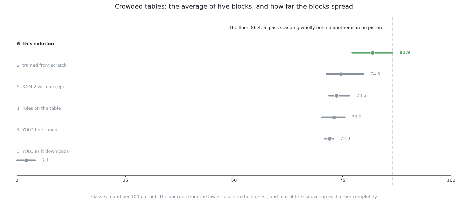
The examiner scored it on five blocks of 20 held-out arrangements. The table below gives its row. Each count is per 100 glasses. The brackets give the lowest and highest block.
| layouts | found per 100 | missed | merged | place | mask covered | mask not the glass |
|---|---|---|---|---|---|---|
| spawned | 96.4 (94.9–98.0) | 3.6 | 0.0 | 6.0 mm | 96.6% | 0.0% |
| crowded | 81.9 (77.2–86.5) | 18.1 | 1.4 | 0.5 mm | 97.2% | 0.0% |
On crowded layouts it is the best of the six. Even its worst block, 77.2, is above the average of every other solution. The best possible crowded score is 86.4, so it is about four and a half glasses short of that. On spawned layouts the fine-tuned YOLO does better, with 99.4. The results set all six side by side and say which gaps are real.
The strengths come first. Each one is explained in full in how it works.
- It answers the question asked. The problem asks which pixels belong to which glass. The output is one mask per glass, with nothing to convert.
- It separates glasses whose outlines join. Two such glasses fill two slots, so nothing has to decide where to cut.
- It has one fewer number to choose. There is no overlap setting for duplicates, because of set prediction. A score cut-off remains, but its meaning is plain.
- It is the only one of the six that can be asked for the hidden part of a glass. This comes from its shape. The second way changes only the target.
- Its licence is permissive. Apache 2.0 matters when the model must ship inside something else.
The weaknesses come next.
- Its second way is the easiest thing in this set to get wrong. If the asserted pixels are fed into the arithmetic, the answer gets worse. Nothing complains, and the width still looks allowed.
- It needs patient training. The one-to-one matching takes time to settle. The fine-tune must also close the domain gap. Both cost time, not correctness.
- It cannot see a glass that is hidden completely. Neither way can. No pixels means no slot and nothing to check.
- It cannot explain its answers. When arithmetic is wrong, you can print a number and see why. When this model is wrong, you can only study examples. The two checks have to catch its mistakes.
- Its weights are a second copy of the cell. They record what the cell looked like when they were fitted. They must be kept in step with the cell. The borrowed part cannot be made again here.
The next section names the published ideas this solution is built from.
2. The general ideas behind this#
The strengths above come from standard parts of modern object detection. Only a few choices are special to this cell: one class, free labels, grey depth pictures, and the request for whole silhouettes.
Detection as set prediction#
A detector outputs a fixed-size set of answers. Training matches that set to the real objects one to one. So duplicates are trained away, not pruned away. DETR (Carion and colleagues, arXiv:2005.12872) did this first. It finds the matching with the Hungarian algorithm (Kuhn, Naval Research Logistics Quarterly, 1955). That algorithm finds the cheapest complete pairing between two sets. It is a general tool, not a vision method.
It suits crowded scenes, because two overlapping objects do not compete. It is a poor choice when a picture can hold more objects than there are slots. It is also a poor choice when training time is short. For more, see object detection.
Attending to a few places rather than everywhere#
If every query looks at every position, reading a picture is slow. So each query looks at a few positions it chooses. Deformable DETR (Zhu and colleagues, arXiv:2010.04159) brought this in. It also works at several scales at once. This made the family practical and sped up training. Later work, such as DINO (Zhang and colleagues, arXiv:2203.03605), makes the matching settle faster and the model run in a fixed short time.
Nearly every current transformer detector uses it. It is not needed when every object is about the same size in every picture. That is not true here. The same glass fills a small patch from the top and much of the picture from the side.
A mask per query, over the whole picture#
Stop painting masks inside boxes. Give each query a short description of its object. Describe every pixel. The mask is the pixels whose description matches the query. MaskFormer and Mask2Former (Cheng and colleagues, arXiv:2107.06278 and arXiv:2112.01527) set this out. They showed that one model of this shape can do several kinds of segmentation. Only the training target changes.
It is the right shape when objects of one class touch and must be reported apart. It is also right when a mask may need to reach past the visible object. That is why it was chosen here. It is not worth it when one map of classes is enough.
Transfer learning and fine-tuning#
Take a model fitted on a large general task. Keep its weights, change its last part, and keep training on the new data. What fine-tuning is explains why this works. Yosinski and colleagues (arXiv:1411.1792) measured how much transfers. Such weights are often fitted on COCO (Lin and colleagues, arXiv:1405.0312). Some are fitted without labels at all, as in DINOv2 (Oquab and colleagues, arXiv:2304.07193). Recent detectors in this family prefer that route.
It is used when labelled data is scarce, which is almost always. It is a weaker choice when labels are free and the new pictures look nothing like the old ones. A network trained from scratch makes that argument. This solution takes the other side on purpose. For more, see transfer learning.
Amodal segmentation#
Amodal segmentation marks the whole object, including the part another object covers. Li and Malik posed it as a task (arXiv:1604.08202). Zhu and colleagues gave an earlier version over whole scenes (arXiv:1509.01329). Later work predicts the visible mask and the whole mask side by side (Follmann and colleagues, arXiv:1804.08864).
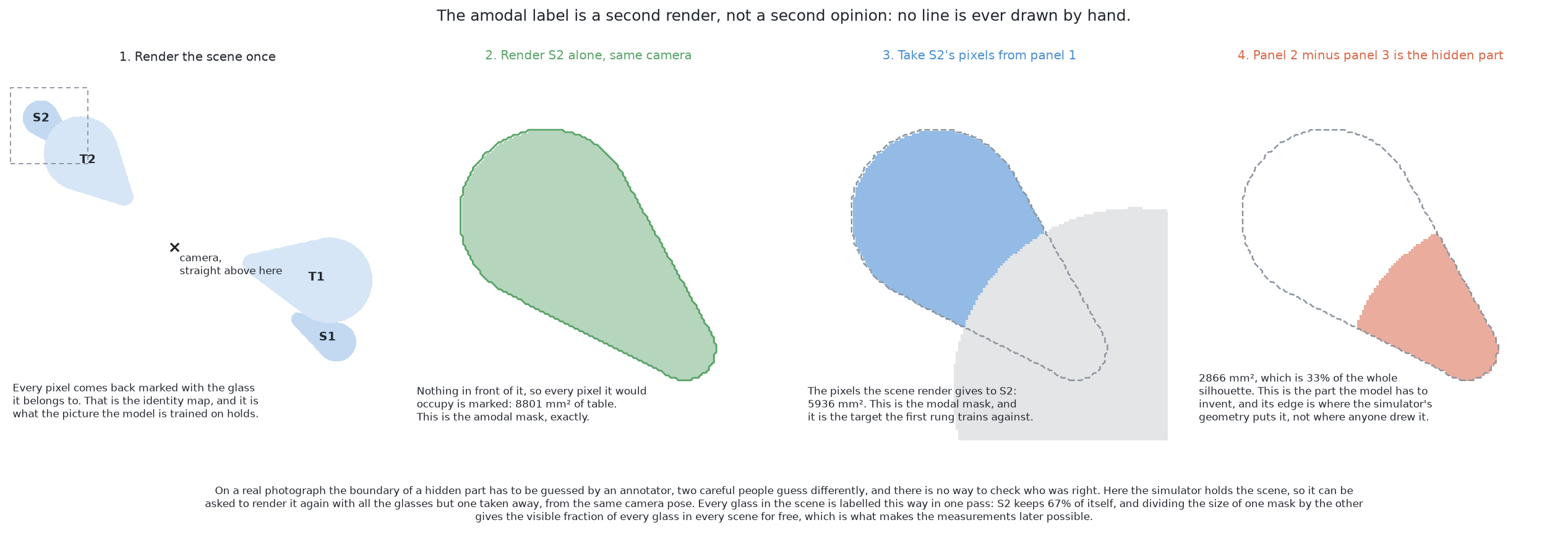
It is used in robot picking, in driving, and wherever a partly covered object must be treated as whole. On real photos it is hard. A person must draw a boundary nobody can see, and two people will draw it differently. A simulator has no such problem. The examiner can draw the scene again without the other glasses. The mask it gets is the exact whole silhouette. For more, see image segmentation.
With the ideas named, the last section places this solution among the other five.
3. Where it sits among the other five#
The ideas above explain what this solution is. This section says what it trades against each of the others. The full scores and which gaps are real are in what the comparison says.
- The same YOLO fine-tuned here. Both are trained the same way, so only the model design changes. That solution wins on spawned layouts and this one wins on crowded ones. This solution also has no rectangle round each mask, and its licence is Apache 2.0 rather than the AGPL.
- YOLO as it downloads. Two things change at once, training and design. So this pair is a rough comparison.
- SAM 2 with a keeper. That solution borrows more and trains less. Its segmenter never sees this cell's pictures. This solution trains the whole model on them, and scores higher on both layouts.
- A network trained from scratch. That solution owns every weight and keeps a small file. It separates glasses by counting votes after the network. This solution gets separate glasses straight from the model, but needs a large borrowed file.
- Rules on the table. On spawned layouts, that solution is better. It finds every glass, needs no training, and can explain its failures. On crowded layouts this solution is ahead and merges far fewer glasses. Both need depth.
No solution of the six can find a glass missing from every picture. Looking again at what was hidden answers that with geometry. This solution only moves that limit a little further out. The overview shows all six side by side.