This page explains what happens inside this solution, one part at a time. It follows the code and says what each part of that code does.
Contents#
- What a transformer segmenter does differently
- Why that matters for this problem
- One class
- Set prediction
- Fine-tuning this model here
- A second way — training against the whole silhouette
1. What a transformer segmenter does differently#
Everything else on this page depends on one difference in the model's shape. So this section explains that difference first.
The older shape is "propose, then refine". The model first proposes rectangles that might hold an object. Then it takes each rectangle on its own. It decides what is inside, tightens the rectangle, and paints a mask inside that rectangle only. The mask is drawn on a small grid and stretched to the rectangle's size. So it cannot reach past the rectangle's edge. The list of proposals starts long and is then cut down in a separate step.
This model's shape is a fixed set of slots. It has a fixed number of queries. A query is a short list of numbers. The model updates it while it reads the picture. Each query asks one question about the whole picture: is there an object, and which pixels are it? The number of queries is set before training. It is larger than the number of objects any picture should hold.
A programmer can think of it like this. The older shape is a list that grows and is then pruned. This shape is a fixed-size array of optional values. Each slot holds one object or is empty. The array has the same length for every picture. A picture with two glasses and a picture with six glasses give arrays of the same length. Only the number of filled slots differs.
The masks follow from that. Each filled query is turned into a short description of its object. Separately, the model describes every pixel. The mask is the set of pixels whose description matches the query. This is worked out over the whole picture. So there is no rectangle for a mask to escape. The model does also report a rectangle for each object. But that rectangle is worked out from the answer. It does not limit the mask.
The next section says why this difference matters for glasses.
2. Why that matters for this problem#
The slot shape from the section above helps in two ways here. The first helps now, and the second is what the second way depends on.
First, two glasses whose outlines join are two different slots from the start. The queries look at the whole picture at once. So nothing ever treats the joined region as one thing, and nothing has to cut it. Two masks come out. They may overlap, because each mask is about a different glass.
Second, a mask has room to grow. Take a glass partly covered by the glass in front of it. The camera sees only one side of it. So the smallest rectangle round the visible pixels is smaller than the glass. In the older shape, the mask is painted inside that rectangle, so it is cut off at its edge. The picture below measures this on one glass of this cell. Of the hidden part of the glass, 61% falls outside that rectangle. So a mask painted in the rectangle could cover at most the other 39%, however it was trained.
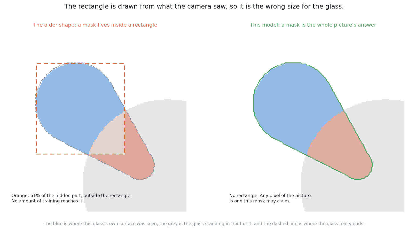
This model has no such edge. A mask may claim any pixel in the picture. So the model can be asked for the whole shape of a glass without any change to its design. That request is the second way. It is the reason this model was chosen for this place in the set.
Before training can be described, one small change to the model must be stated. The next section gives it.
3. One class#
Training needs a list of classes, so this section says what the list is here. The same YOLO fine-tuned here makes the same change.
A borrowed detector knows a long list of everyday objects. Here that list is replaced by one entry, "glass". So each query only chooses between "glass" and "nothing". The model is no longer asked what kind of object it found. It is asked only whether it found one, and which pixels it is.
This has one gain and one loss. The gain is that the model cannot call a glass a vase. The loss is that a high score now means only "something is here". It does not say which kind of glass. That does not matter here, because the kind on the table is known. It would matter if several kinds stood on the table together.
One class does not make the model much smaller or faster to train. Almost all the weights are in the part that reads the picture. That part does not know about the class list.
With slots and one class in place, the next question is how training gets one answer per glass. The next section answers it.
4. Set prediction#
The slots from the first section need a way to avoid two slots reporting the same glass. This section explains how training does that.
Set prediction means the model's whole output is one set of answers. It is compared with the set of real glasses. At each training step, the filled slots are matched to the real glasses one to one. Each real glass gets exactly one query. Each query gets at most one glass. The pairing chosen is the one that fits best overall. Every query left over is told its answer should have been "nothing".
This has one important result. Suppose a query reports a glass that another query was already matched to. It gets no credit for being nearly right. It is told it should have said "nothing". So training removes duplicate answers from the model itself. A picture with four glasses comes back with four filled slots, because that is what training rewarded.
The older shape works differently. Several proposals land on one object, because several nearby rectangles all hold most of it. All of them score well. So a separate step must reduce them to one answer. It sorts the claims by score, keeps the best, and drops every claim that overlaps it by more than a set amount. Then it repeats. This step is called non-maximum suppression. It has one setting, which is how much overlap counts as a duplicate. It also assumes that heavy overlap means a duplicate.
In this cell that assumption causes less trouble than you might expect. Splay makes one glass's outline spread across another's, so different glasses do overlap. But they do not overlap enough to be dropped. Take the pair that overlaps most. These are two glasses of the tall, wide end of the kind, on a line out from the camera. Stand them as close as the examiner's crowded arrangements ever do. Their two rectangles then share 0.48 of the area they cover together. The fine-tuned YOLO's pruning step uses 0.7.
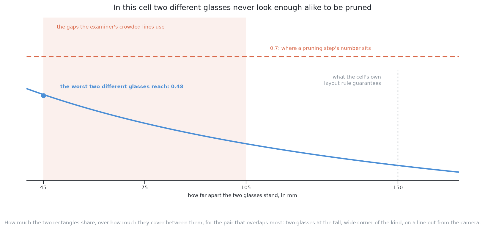
So the setting does not drop glasses today. But somebody had to choose it with this geometry in mind. They would have to choose it again if the camera moved, the survey height changed, or a taller kind came to the table. Set prediction removes both the setting and the assumption. There is no overlap amount to choose. Two overlapping glasses never compete, because each has its own slot.
Set prediction has a cost too. Training must match slots to glasses before it can score anything. Early in training, the glass a query is matched to can change from step to step. So models of this family need patient training. Much of the published work on them is about making the matching settle faster.
The design is now complete. The next section is about where its weights come from.
5. Fine-tuning this model here#
The sections above described the model's shape. This section says how its weights are set for this cell.
The model starts from weights fitted to a large set of ordinary photos. Training then continues on this cell's pictures. This is fine-tuning. Most of the borrowed weights already work, so they need only small changes. That is why a few hundred pictures are enough for a model this size. What fine-tuning is explains this in full.
The labels cost nothing. The examiner already knows which glass owns each pixel, so every mask comes from that. What the examiner draws explains this. The model is never tested on an arrangement it trained on.
The pictures are grey depth pictures, not photos. The borrowed weights were fitted to colour photos. This difference is called the domain gap. Why it failed explains it. Fine-tuning does not remove the gap. But the model is trained on the same grey pictures it will see later. So the gap should cost accuracy and training time, not correctness. This is a reasoned expectation, not a measured result.
The training arrangements need one deliberate choice. The cell's own layout rule keeps glasses well apart. A model trained only on those would never see a hard pair. So half of every training set uses crowded arrangements. These stand glasses closer than the rule allows, on lines out from under the camera. The lesson is general. Train the model on cases harder than any it must handle.
The first way is now fully described. The next section describes the second way, which only this solution can offer.
6. A second way — training against the whole silhouette#
The missing rectangle from the second section makes a second way of training possible. This section explains it.
The idea fits in one sentence. Train each mask against the glass's whole silhouette, instead of only the pixels the camera can see. The silhouette is the shape the glass would have if nothing stood in front of it. A mask of the visible part is called a modal mask. A mask of the whole silhouette is called an amodal mask. The amodal mask always contains the modal one. The difference between them is the hidden part.
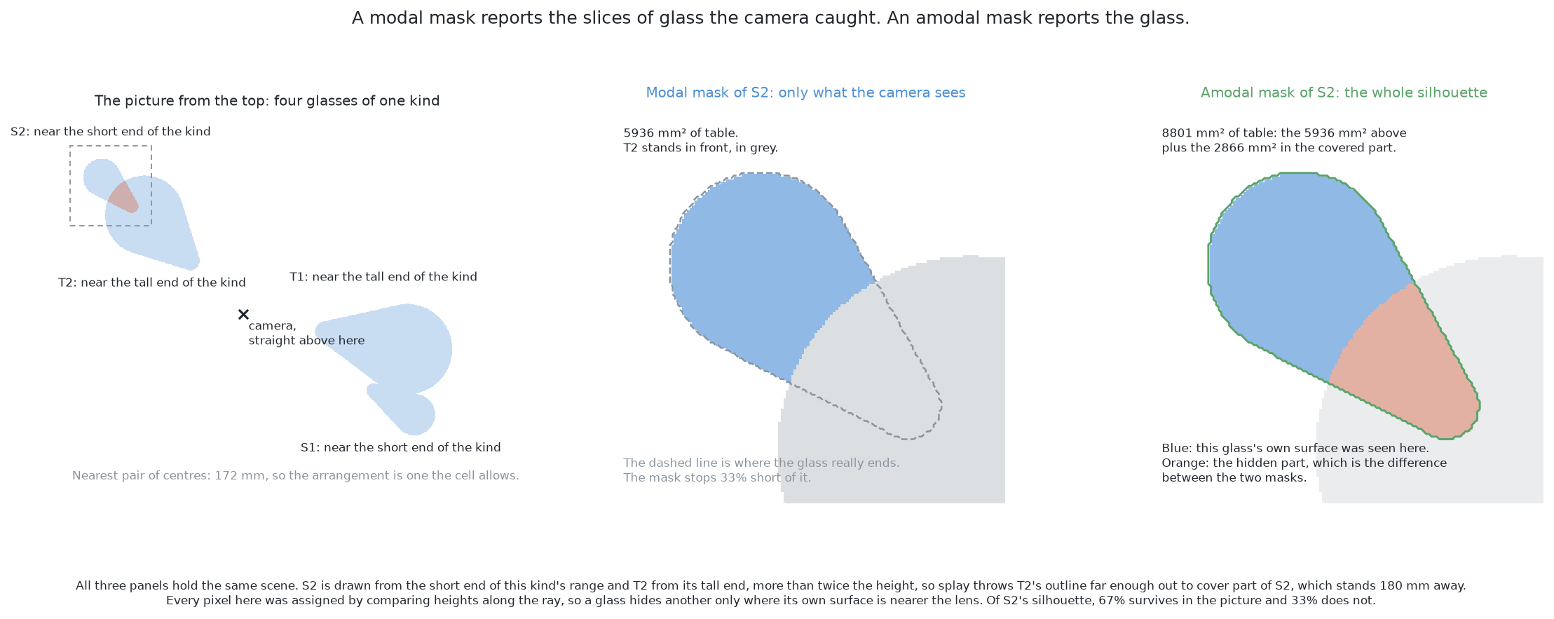
It matters because the failure it answers gives no warning. Put one glass partly behind another. A mask of visible pixels loses everything behind the near glass. What is left is a slice along one side. The shared arithmetic reads that slice as a narrower glass. Nothing objects, because the kind's footprints run from 65 to 105 mm. So a short width still looks allowed. A slice does not look like an error. It looks like a smaller glass.
Compare that with two glasses that come back as one region. Then the width is too large for the kind. The check fires, and the region is marked as doubtful. So a merge is caught, but a slice is not. The worked example measures how much room the slice has.
The model's design suits this request. Asking for the whole silhouette changes only what the mask is scored against. The model's shape does not change. This is a general lesson: one network can answer a different question by changing its target, not its shape. The task is still hard. The model must learn the shape of the kind. It must also tell which glass is in front.
One rule has no exceptions. A mask that claims pixels the camera never saw the glass at must name those pixels. The depth reading there belongs to the glass in front. How a mask becomes a record measures what goes wrong otherwise.
The simulator gives two checks on such a model for free. First, on a glass with nothing in front of it, the amodal mask must equal the modal one. So you can measure what the model adds to uncovered glasses. A model that adds a little everywhere will show up. Second, during training, watch the overlap over the hidden part alone. The examiner can supply it by taking one of its masks away from the other. Do not use overlap against the visible truth. Every correct pixel of a completion lies outside that truth, so that score punishes the model for working. A score that rewards doing nothing will be won by a model that does nothing.
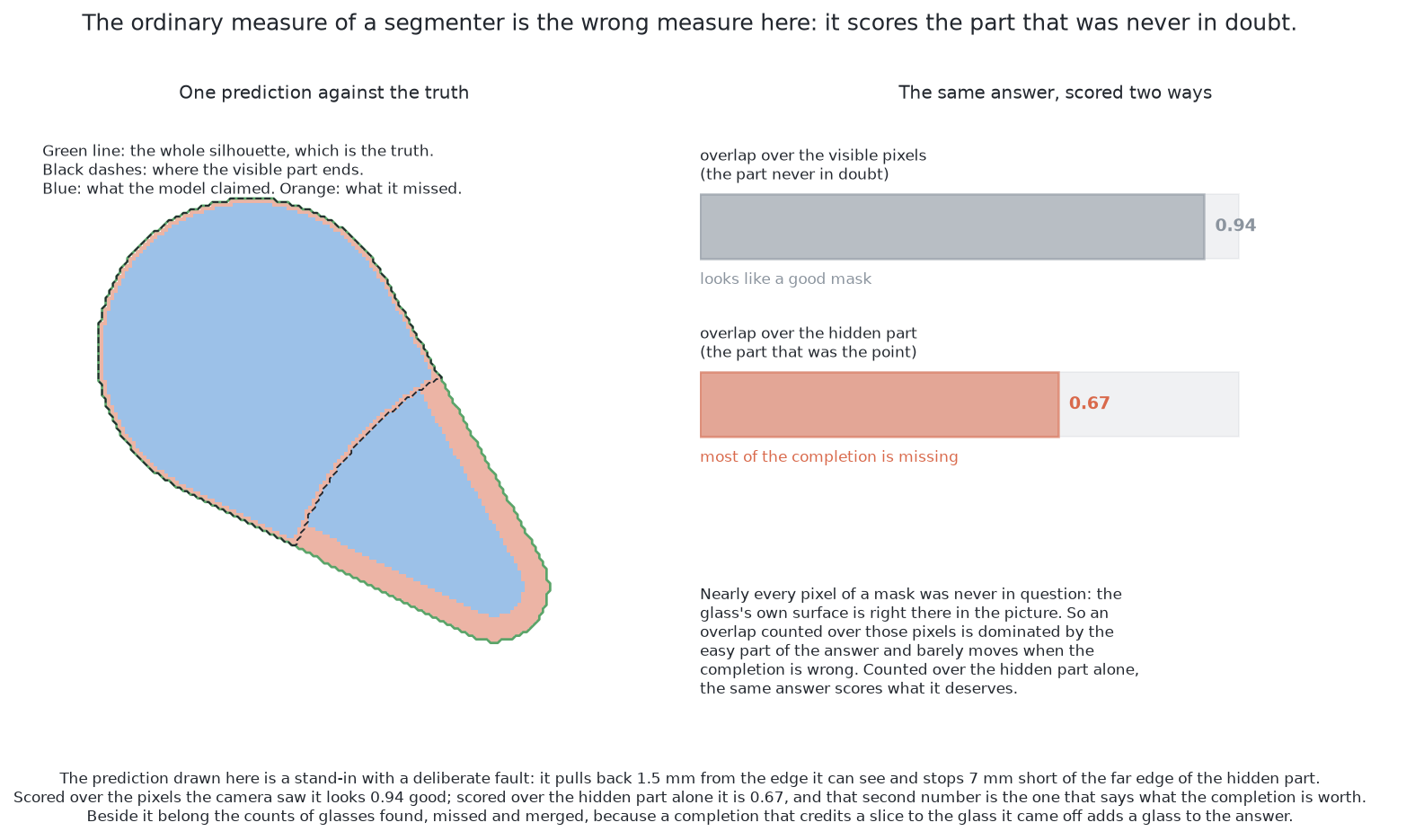
This way was never fully trained, so it claims no number. Its training reached four epochs of ten, and its check score was still rising. Other training runs filled the machine, and it was stopped. So this section is a design, not a result. This solution's row in the results is the first way.
A worked example now follows both ways through one arrangement.
← The code · A worked example →