How the model is trained

This page explains the training step in detail. It says what goes in, which library does the work and why, and what each part of the training call asks for. It follows the code, which shows the training step in three numbered steps. This page takes those steps one at a time. Every file it names is in the solution's folder on GitHub.

Contents#

1. What fine-tuning is
2. The inputs: scenes, pictures and label files
3. The library: Ultralytics
4. Loading the borrowed weights
5. The training call, argument by argument
6. What the run did, and what it produced
7. Two ways training on one cell's pictures goes wrong

1. What fine-tuning is#

The code calls one method to train the model. So it helps to say first what that method does.

A weight is one of the numbers inside a model. Training a model means three things. Show it an example. Compare its answer with the right answer. Then change every weight a little, in the direction that would have helped. Training from a random start means the weights begin as noise. Training then has to build every part of the model from nothing. Fine-tuning means the weights begin at values from somebody else's training. So training has much less to do.

The saving comes from the early layers of the model. These layers react to things that all pictures have, such as edges and corners. A grey picture shaded from depth has many edges. For example, the rim of a glass against the table is a big jump in distance, so it is a big jump in grey. So the early layers work here almost unchanged. The later layers decide what an object is. They were fitted to the colours and textures of photographs. This cell does not draw colour or texture. So training has to change those later layers. Yosinski and colleagues measured this (arXiv:1411.1792). The deeper a layer is in the network, the worse it transfers to a new kind of picture.

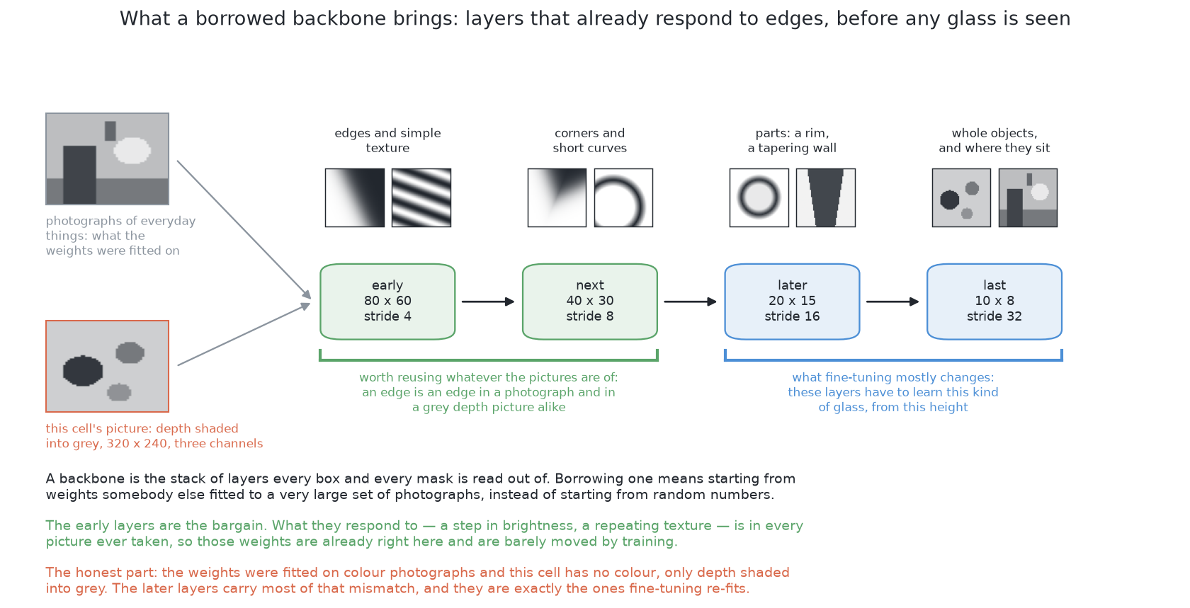
Now we know what training changes. The next question is what the model is shown, because the library cannot read the examiner's scenes directly.

2. The inputs: scenes, pictures and label files#

This section covers step 1 of the training step in the code. The inputs must be on disk before training can start.

The scenes. dataset.scenes in dataset.py picks the arrangements to train on. Half are spaced, as the cell's own rule spaces them. Half are crowded closer than that rule allows. The crowded half shows the model pairs of glasses that are hard to separate. Spaced scenes alone would never show it one. The examiner has a dividing line. Arrangements below it are for training. Arrangements above it are for marking. Every training scene comes from below the line. Two checks refuse a scene from above it: one in data.training_seeds and one in dataset.write.

The split. fit holds every fourth scene back. The training run checks its own progress on these pictures, which it is not trained on. The scenes arrive spaced first and crowded after. So taking the last quarter would give crowded scenes only. Taking every fourth scene gives both kinds. These held-back scenes are not the examiner's marking arrangements. Both parts come from below the dividing line.

The pictures. Each scene is seen from three survey stations, so each scene gives three pictures. dataset.write saves each one as a PNG file. The picture is the same grey picture shaded from depth that every solution gets. It is 320 pixels wide and 240 high. The grey is copied into all three colour channels.

The label files. Beside every picture, dataset.write saves a text file with the same name. It has one line per glass. A line starts with the class number, which is always 0. Then it lists the corners of the glass's outline as pairs of numbers. Each corner is a fraction of the picture's width and height. So a corner in the middle of the picture is 0.5 0.5. The first picture in the training set is crowded-00050-station-0. It has four lines, with 151, 106, 154 and 29 corners. Its first line begins like this:

0 0.112500 0.491667 0.109375 0.495833 0.100000 0.495833 ...

The outlines come from the examiner's id image. This image marks each pixel with the glass it shows, or with nothing. dataset.label turns one glass's pixels into an outline with three rules:

• It skips a glass that has fewer than 100 pixels in this picture. The shared arithmetic uses the same limit. Below it, there is too little of a glass to measure.
• It keeps only the largest connected piece of a glass's pixels. Something in front of a glass can break its visible pixels into patches. Each line of a label file is one object. So writing every patch would teach the model that one glass is several glasses.
• It labels only the pixels the camera saw, not the whole outline. A glass partly behind another is labelled with the slice that showed. Training towards the whole outline is solution 6's choice.

A picture with no glass in it is still written, with an empty label file. The model has to learn that the answer there is nothing.

These labels cost nothing here, because the simulator draws them. The examiner explains this. On real photographs, a person would draw every outline by hand.

The description file. Last, dataset.describe writes a small YAML file. YAML is a plain-text format for settings. The file says where the two parts are and what the classes are called. The run's file looks like this, with the full path shortened:

# Written by dataset.py. One class, which is the point of this solution.
path: .../04-yolo-fine-tuned/dataset
train: images/train
val: images/val
names:
  0: glass

The names list holds the one class. The borrowed model knows 80 everyday categories. This file names only one. So the model is not asked which everyday object it sees. It is asked only where the objects are. This removes the naming failure of solution 3.

dataset.build empties the folder before it writes. Ultralytics keeps a cache of the labels it reads. Without this, a new set written over an old one could be trained on the old labels, with no warning.

The inputs are now on disk. The next section introduces the library that reads them.

3. The library: Ultralytics#

The last section wrote the inputs in one fixed format. This section says whose format it is, and why this solution uses it.

What it is. Ultralytics is a Python package. It holds the YOLO models and the code to train them, run them and measure them. It runs on PyTorch. On this machine, PyTorch uses the built-in graphics through MPS. MPS is PyTorch's way of using the graphics processor on an Apple machine.

What it does for you. It runs the whole training loop. You give it the YAML file and a starting weights file. Then one call does all of this:

• reads the pictures and labels;
• rebuilds the model's last layers for the new list of classes;
• chooses an optimiser, which is the rule that turns an error into a change of weights;
• changes the pictures a little as it goes;
• checks itself after every pass;
• keeps the best weights.

So the training is one line of this solution's code.

Why this one rather than the obvious alternative. The obvious alternative is to write the training loop by hand in PyTorch. Solution 2 does this for its own small network. Here, that would mean writing the loss for boxes and masks, the matching of predictions to labels, and the measuring, all again. The main reason is the matched pair. Solution 3 uses this library and this weights file unchanged. This solution must differ from it only in the training. Using the same library's own training method keeps everything else the same.

What it costs. There are three costs.

• It reads a training set only from a folder in its own format. That is why dataset.py exists.
• Defaults that the code never names decide most of the training. For example, they choose the optimiser and how the pictures are changed. The run records all of them in runs/fine-tune/args.yaml. What the run did reads the important ones.
• Its licence is the AGPL-3.0. This solution makes a new weights file by training the borrowed one further. A file made from an AGPL work has the same terms. So the trained file also falls under the AGPL, and this project does not own it outright. Solution 3's page explains what the AGPL asks.

The Ultralytics training guide lists every setting. Its page on segmentation datasets describes the label file format. Both open in a new tab.

The library's first job is to load the starting weights. The next section describes this.

4. Loading the borrowed weights#

Step 2 of the training step starts by loading the model. This section shows where that file comes from.

model = YOLO(str(borrowed()), task="segment")

borrowed() is in yolo_fine_tuned.py. It returns the path of yolo26n-seg.pt, the smallest YOLO26 segmentation model. It calls Ultralytics' attempt_download_asset. This downloads the file on the first run and finds it on disk after that. The file is kept in the solution's own weights/ folder, not in the home directory. So deleting that folder starts everything again. Solution 3 names the same file. The solution's README says that a test checks the model is named in one place only.

YOLO(...) builds a model object around those weights. task="segment" asks the model to return outlines as well as boxes. Nothing is trained yet. At this point the object is exactly solution 3's model, with its 80 categories.

The next section is the line that turns it into this solution's model.

5. The training call, argument by argument#

The model is loaded and the inputs are on disk. Now the training is the one call below. This section reads it one argument at a time.

model.train(
    data=str(described),
    epochs=epochs,
    imgsz=PICTURE,
    batch=BATCH,
    device=device.pick(),
    project=str(Path(__file__).parent / "runs"),
    name="fine-tune",
    exist_ok=True,
    workers=0,
    seed=FITTING_SEED,
    deterministic=True,
    plots=False,
    verbose=False,
)

In the table below, the first column is the argument. The second is the value the marked run used. The third says what the argument asks for.

Two important values do not appear in that call. The first is the number of classes. train reads the YAML file and finds one class. The loaded model has 80. So it builds a new model with one class. It then copies in every borrowed weight whose shape still fits. That is every weight except the layer that scores the classes. That layer has one row per class. Ultralytics would copy a row if a borrowed category had the same name. None of the 80 is called "glass", so that row starts from nothing.

The second missing value is the confidence bar. Training does not use it. It is used later, when the trained model answers. It stays at solution 3's 0.25. The overlap allowed between two candidates also stays at solution 3's 0.7. Changing either would be a second difference between the pair. Then its effect could be mistaken for the effect of training.

When the call returns, model.trainer.best is the path of the best weights the run kept. Step 3 copies that file to weights/fine-tuned.pt. run.py loads this file for marking. model.trainer.metrics holds what the run measured on its held-back pictures. fit returns it, together with counts of what went in.

The call names only a few settings. The library chooses the rest. So the next section reads what the library chose and what came out.

6. What the run did, and what it produced#

This section uses the run's own record, runs/fine-tune/args.yaml, and the Ultralytics source code. Together they show what happened inside the call above. The run was started with train.py --scenes 100 --epochs 60.

What went in. There were 100 scenes, 50 spaced and 50 crowded. The model trained on 75 of them. That is 225 pictures with 1034 outlines. The other 25 scenes, 75 pictures, were held back for the run to check itself.

The optimiser it chose. The setting was left at auto. Ultralytics then counts how many weight changes the run will make. It adds up the errors from eight batches of eight pictures before it changes any weight. So each change uses 64 pictures. 225 pictures give about four changes per pass. Over 60 passes, the library counts 240 changes. Below 10,000 changes, the library chooses AdamW. AdamW is a common optimiser that sets how far each weight moves. Its learning rate depends on the number of classes. For one class the rate is 0.002. In the first few passes, the rate rises slowly from almost zero. This stops the new, random class row from pulling the borrowed weights about.

How it changed the pictures. Ultralytics changes every training picture a little each time it shows it. Then the model cannot learn one picture by heart. The run used the defaults. It flipped pictures left to right half the time. It moved and resized them. It changed their brightness. It joined four pictures into one mosaic. For the last 10 passes it stopped making mosaics. So the model ends on pictures shaped like the ones it will really see.

How it chose the best weights. After every pass, the run measured itself on the 75 held-back pictures. The measure is the mean average precision, or mAP. It scores how well the predicted outlines match the labelled ones. The run kept the weights from the pass with the best mAP for masks and boxes together. It saved them as best.pt.

What came out. The run took 39 minutes. At the last pass, its mAP for masks was 0.995 on its held-back pictures. Here an outline counts as right when it overlaps the label by at least half. That number is not this solution's score, because those pictures come from below the dividing line. It only shows that training settled. The marked score is on the results page.

A short run is not enough. The defaults in train.py are 16 scenes and 10 passes. That run finishes in 52 seconds. But its model never gives a candidate a score above 0.02. So at the bar of 0.25 it finds nothing at all. The class row starts from nothing. It needs real training before its confidence can pass the bar.

Training this long on one cell's pictures has its own risks. The last section names them.

7. Two ways training on one cell's pictures goes wrong#

The run above trained hard on a narrow set of pictures. That is where the two usual risks of fine-tuning come from.

Catastrophic forgetting. Training a model further on a narrow set of pictures moves its weights away from what they knew. The model gets better at this cell and worse everywhere else. In this project that costs nothing, because the model only ever sees this cell. But the weights file must then match the cell. Solution 2's needs explains this cost.

Overfitting. A model trained on a small set can learn the examples instead of the idea. Here it could learn the arrangements instead of the glasses. Two things guard against this. First, the examiner marks a solution only on arrangements it was not trained on. So overfitting shows up as a lower score. Second, the labels are free. So the training set can be made larger, and the only cost is rendering time.

Both risks grow with more training. The domain gap shrinks with more training. The domain gap is the difference between the pictures a model learned on and the pictures it is shown. So there is a sensible amount of training, not a maximum. The marking arrangements decide it. The next page gives what they said about this run, and compares the result with the other five solutions.

← The code · Results and comparison →