The page before this one, open-vocabulary vision, ended by grounding the phrase "the mug behind the bowl". It could only do that by subtracting one measured distance from another. Those distances had to come from somewhere, because the pictures on that page were flat and a flat picture holds no distances at all. This page is about where they come from.
The gap matters more for an arm than for anything else a camera is pointed at. A program that sorts photographs needs to know what is in them. A program that drives a gripper needs to know where things are, in millimetres, because the fingers have to close around an object rather than in front of it or behind it.
This page covers three ways of measuring distance and three ways of holding the result. By the end of it you will understand what a depth picture is, how a network guesses distance from a single photograph and why that guess has no true scale, what a pair of cameras measures and how accurate the measurement is, why a depth camera that throws a pattern of dots fails on glass, how a depth picture becomes a cloud of points, and what a learned description of a whole scene buys a robot.
The page is written for a reader who has read open-vocabulary
vision and vision
backbones, and who has met point clouds on pictures,
sound and robot
states.
The only maths used is multiplying, dividing and subtracting. Every number in
every picture is worked out by docs/diagrams/models_that_see_2.py, and the
script prints each number when it runs. The camera arithmetic is real. Where a
scene had to be invented, the script makes it with a fixed random seed and this
page says so.
Contents#
- A flat picture has no distances in it
- Guessing depth from one picture
- Relative depth and metric depth
- Two cameras, and the arithmetic of the shift
- Cameras that throw a pattern, and the surfaces that defeat them
- From a depth picture to a shape the arm can use
- Learned scenes: radiance fields and splatting
- Where to read next
- Using it in Python
1. A flat picture has no distances in it#
The last page treated a picture as a grid of brightness values, which is what a picture is. The first thing to see is what that grid leaves out. A camera lens turns each direction it gathers light from into one pixel. A pixel therefore records which direction the light came from, and it says nothing about how far along that direction the surface was. The picture below shows one pixel and three of the places that could have produced it.
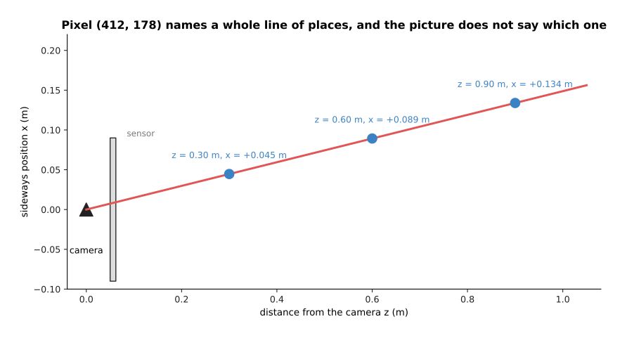
With a lens of focal length 615 pixels, pixel 412, 178 means the point 0.045 metres sideways at a distance of 0.30 metres, or 0.089 metres sideways at 0.60 metres, or 0.134 metres sideways at 0.90 metres.
Every one of those places would make exactly the same pixel. That is true of every pixel in every photograph ever taken. What a robot needs is therefore one more number for each pixel, saying how far along its direction the nearest surface sits. A grid that holds one such distance for every pixel is called a depth map. The small depth map below stands for a sloping table with a mug on it, and each cell carries its own distance in millimetres.
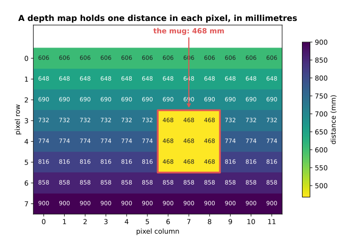
The table's distance grows from 606 millimetres at the top row to 900 at the bottom row, while the nine cells of the mug all read 468, because the mug stands closer to the camera than the table behind it.
A depth map is stored exactly like a grey photograph, as one number per pixel. Most of the tools built for pictures therefore work on it unchanged, and the only difference is that the number is a distance rather than a brightness. That difference changes what the picture is useful for. The picture below takes one row of an invented scene and plots it twice: the upper chart is brightness along that row, and the lower chart is distance along the same row.
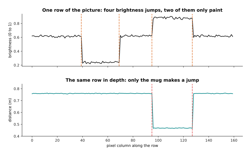
Along one row of this simulated scene the brightness jumps at columns 39, 69, 95 and 127, while the distance jumps only at 95 and 127, because the first two brightness jumps are a stripe painted on a flat table.
That picture is the reason a depth map is worth having at all. A painted line, a shadow and a printed label all make brightness jump where nothing changes physically. A program looking for object edges in a photograph therefore finds edges that are not there. In the depth map only the mug makes a jump, because only the mug sticks up. The two kinds of picture make different mistakes, which is why a robot wants both, and the rest of this page is about how the second one is produced.
2. Guessing depth from one picture#
The cheapest way to get the depth map that section 1 asked for is to guess it from the photograph you already have. The guess is made by a network trained on pairs of photographs and measured depth maps. Such a network works surprisingly well, and it has one limit that no amount of training removes. The picture below shows the limit.
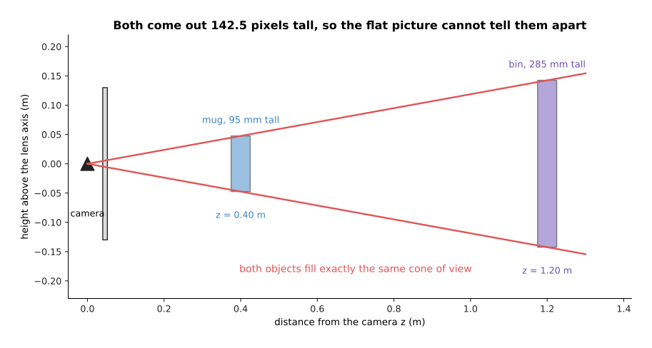
Through a lens of focal length 600 pixels, a mug 95 millimetres tall at 0.40 metres and a bin 285 millimetres tall at 1.20 metres both come out 142.5 pixels tall, because three times the size at three times the distance fills the same cone.
The arithmetic is one line. The height of a thing in the picture is the focal length times its real height divided by its distance. So 600 times 0.095 divided by 0.40 is 142.5, and 600 times 0.285 divided by 1.20 is also 142.5. The picture below plots that one line for both objects, so that you can see the two curves cross the same height.
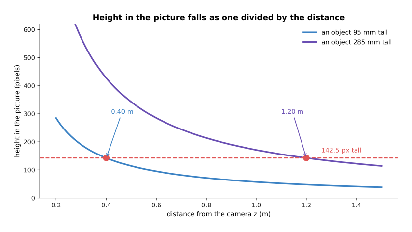
The height in the picture falls as one divided by the distance, so a 95 millimetre object reaches 142.5 pixels at 0.40 metres and a 285 millimetre object reaches the same 142.5 pixels at 1.20 metres.
Nothing in the photograph tells the two cases apart. A single picture can therefore never give a true distance on its own, and any model that returns one is leaning on an assumption about how big things usually are. The picture below shows what that assumption costs. It takes one object 142.5 pixels tall and asks what distance follows from five different guesses at its real height.
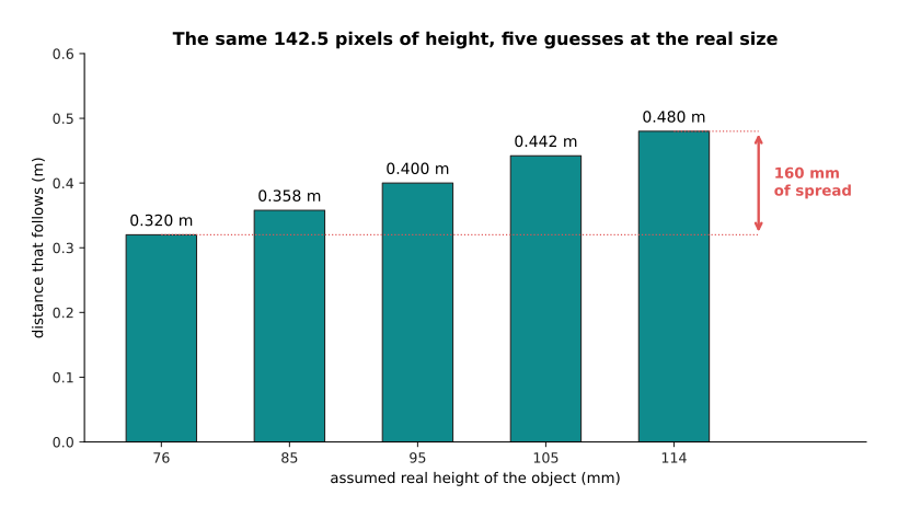
For a thing 142.5 pixels tall, assuming a real height of 76 millimetres puts it at 0.320 metres and assuming 114 millimetres puts it at 0.480 metres, so a twenty per cent spread in the assumed size moves the answer by 160 millimetres.
That assumption is not written anywhere in the model. The model learns it from the training pictures. This is why such models work well on kitchens and offices full of ordinary objects, and badly on a bench covered in parts that have no usual size, and why a doll's house breaks them completely. What the network does get right is the shape of the scene, which means how the surfaces in the scene are arranged relative to each other.
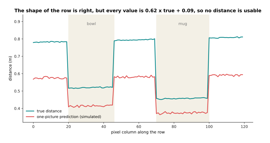
In this simulated row the prediction is 0.62 times the true distance plus 0.09, which puts the mug 83 millimetres too near and the far table 216 millimetres too near, while keeping the near-to-far order exactly right.
A model whose output is right up to one multiplication and one addition is still useful, because the order of the surfaces is preserved. The next section is about what you can and cannot do with such an output.
3. Relative depth and metric depth#
Section 2 produced a depth map that had the right shape and the wrong numbers. This section gives the two kinds of answer their names. A depth map that tells you which surfaces are nearer than which, without being in any unit, is called relative depth. A depth map whose numbers are real distances in metres or millimetres is called metric depth. The difference is not a matter of accuracy, because a relative map is not a slightly wrong metric map. It is a map that has no scale at all. The picture below makes that concrete by reading the same relative map under three different scalings.
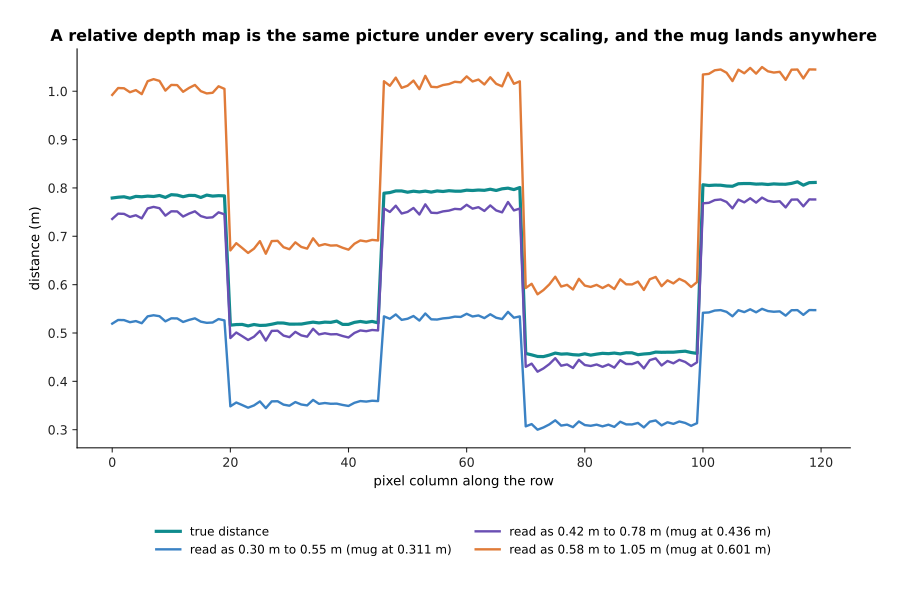
The same relative map read as 0.30 to 0.55 metres puts the mug at 0.311 metres, read as 0.42 to 0.78 metres it puts the mug at 0.436, and read as 0.58 to 1.05 metres it puts the mug at 0.601, and nothing in the map says which reading is right.
To turn a relative map into a metric one you need at least two real distances to pin it to. Those two distances can come from a laser rangefinder, from a stereo camera, or from knowing where the table surface is. A measured distance used this way is called an anchor. You then find the one multiplication and the one addition that carry the predicted values onto the two anchors, and you apply that multiplication and that addition everywhere else. The picture below fits the relative row twice, once from two anchors far apart in depth and once from two anchors that are nearly at the same distance.
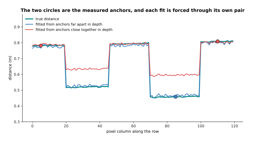
Each fit passes through its own pair of circles exactly, and the fit from the two close anchors then drifts far away from the true distance everywhere else.
The picture below measures how far away. It plots the distance error that each fit leaves behind, against the 6.5 millimetres of room the gripper has.
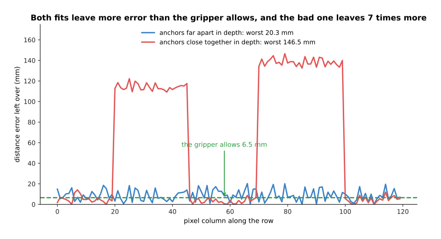
Two anchors 350 millimetres apart in depth leave a mean error of 8.7 millimetres and a worst error of 20.3, while two anchors only 26 millimetres apart leave a mean of 61.6 and a worst of 146.5, which is seven times worse.
The reason the second fit is so much worse is worth stating plainly. The two numbers being solved for are a scale and an offset. Solving for a scale from two points at almost the same distance means dividing by something close to zero. The sensor noise at those two pixels is therefore multiplied up into the answer. Anchors have to straddle the depth range you care about, which means one point on the near object and one point on the far background.
Even the good fit leaves 20.3 millimetres in the worst place, and the picture below says what that means for an arm. It puts the mug's true distance beside four estimates of it.
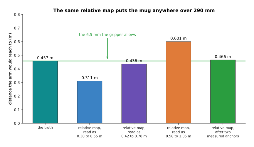
The mug really sits at 0.457 metres, the three readings of the relative map put it at 0.311, 0.436 and 0.601 metres, which is a spread of 290 millimetres, and the two-anchor fit puts it at 0.466 metres, which is 8.5 millimetres out against a gripper margin of 6.5.
So relative depth answers every question about order. It says which object is nearest, it lets you avoid the nearest obstacle, and it resolves the word "behind" in a phrase. It answers no question in millimetres. Metric depth answers both kinds of question. That is why a robot that has to reach needs either a model that returns metres or a second sensor to pin a relative map to. The next two sections are about the sensors that measure distance directly.
4. Two cameras, and the arithmetic of the shift#
Section 3 needed real distances to pin a relative map to, and the oldest way of measuring one is to use two cameras. Two cameras a fixed distance apart, looking at the same scene, are called a stereo pair. The distance between the two cameras is called the baseline. The difference between where a point lands in the two pictures is called the disparity. The whole method is one division, and the picture below shows where the division comes from.
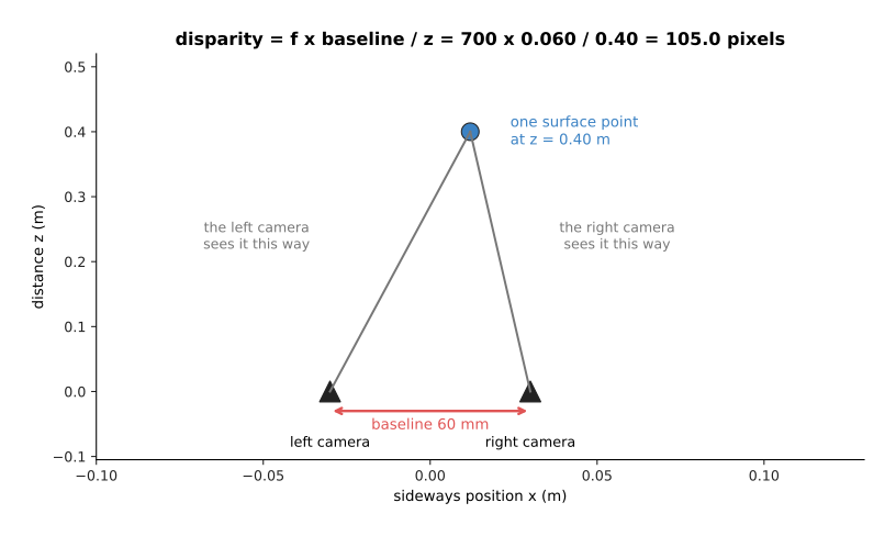
With a focal length of 700 pixels and a baseline of 60 millimetres the disparity is 42 divided by the distance, so a point at 0.40 metres shifts by 105 pixels between the two pictures.
Because the disparity is 42 divided by the distance, it falls quickly as things get further away. The picture below plots the disparity across the whole range.
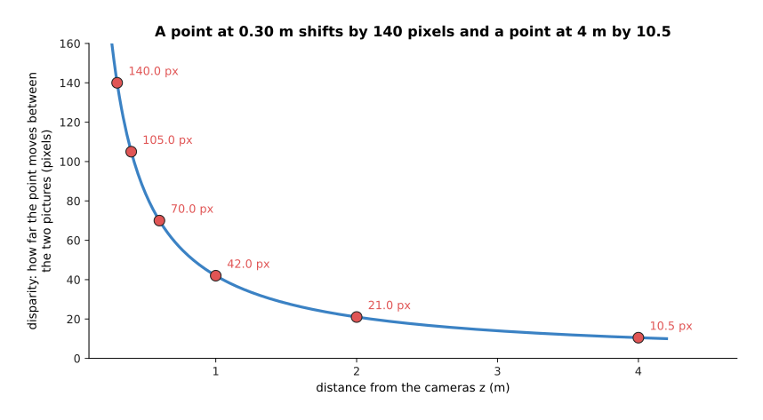
A point at 0.30 metres shifts by 140 pixels, a point at 1 metre shifts by 42, and a point at 4 metres shifts by only 10.5.
Because the disparity falls that way, the measurement error does not stay the same across the room. Suppose the matching is uncertain by a quarter of a pixel. That same quarter of a pixel turns into a distance error that grows with the square of the distance, as the picture below shows.
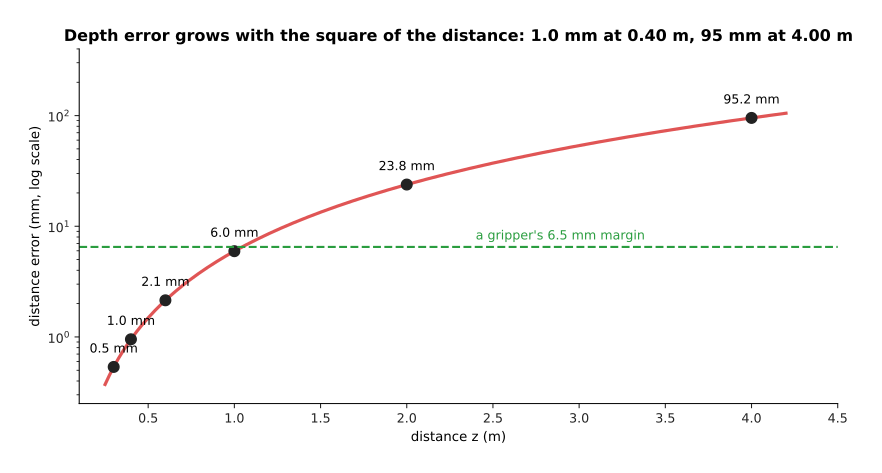
A quarter of a pixel of matching error costs 1.0 millimetres at 0.40 metres, 6.0 millimetres at 1 metre and 95.2 millimetres at 4 metres, so ten times the distance brings a hundred times the error.
That curve explains why a stereo pair is a good choice for a table in front of an arm and a poor choice for the far end of a room. It also says what to do when accuracy is short. Both the baseline and the focal length sit underneath the division, so you can move the cameras further apart or use a longer lens. The picture below shows what moving the cameras apart buys at one metre.
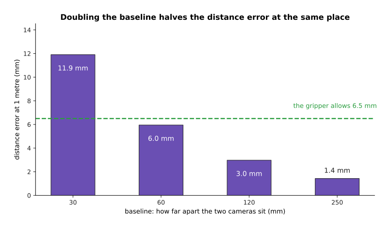
At one metre a quarter of a pixel of matching error costs 11.9 millimetres with a 30 millimetre baseline, 6.0 with 60 millimetres, 3.0 with 120 and 1.4 with 250, so doubling the baseline halves the error.
Widening the baseline is not free, because it costs you the near range. Two cameras far apart stop seeing the same close object at all. The picture below draws the view cone of each camera for two baselines, and marks the nearest point that falls inside both cones.
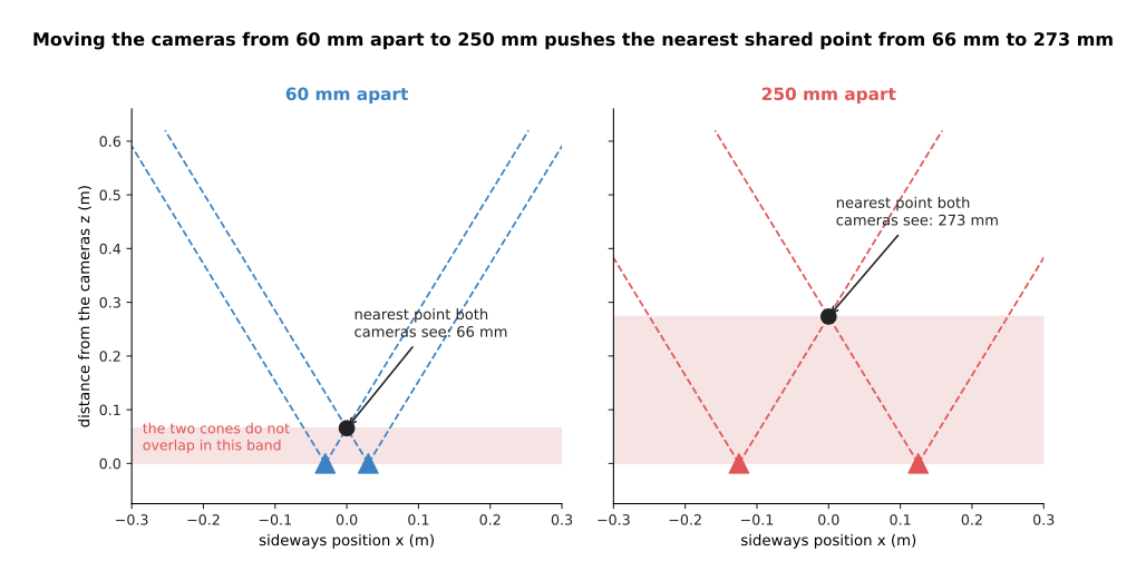
A 640 pixel wide picture taken with a 700 pixel lens covers 49.1 degrees, so a 60 millimetre baseline leaves the two cones overlapping from 66 millimetres outwards, while a 250 millimetre baseline pushes that limit out to 273 millimetres.
The hard part of stereo, though, is not the arithmetic. The hard part is working out which pixel in the right picture is the same surface as a given pixel in the left one. That is only possible where the surface has something to match. The picture below shows one row of the left picture across textured wood and across a plain white wall.
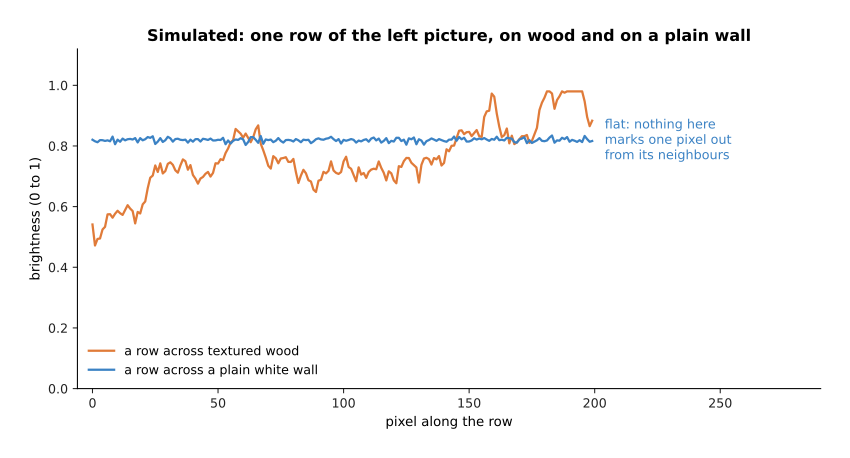
On the simulated wood the brightness changes from pixel to pixel, while on the plain white wall it stays at about 0.82 everywhere, so nothing in the wall marks one pixel out from its neighbours.
Matching works by sliding a small window of the left row along the right row and measuring, at each shift, how badly the two windows differ. The shift with the smallest difference is the answer. The picture below plots that difference against the shift tried, for both surfaces.
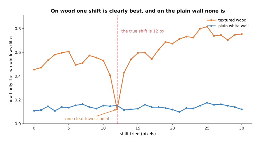
On the simulated wood the best shift is the true 12 pixels and the next-best shift away from it scores 0.335 worse, while on the plain white wall the whole curve spans only 0.078 and the best shift lands at a wrong 21 pixels.
So a stereo camera gives nothing on a blank wall or a plain white table. The common fix is to throw texture onto the scene instead of waiting for it, and that is what the next section is about.
5. Cameras that throw a pattern, and the surfaces that defeat them#
Section 4 ended with stereo failing for want of texture, and the fix is to add some. A depth camera of this kind shines a pattern of infrared dots onto the scene and measures where each dot lands. It measures the landing place either with a second camera or by comparing against the pattern it sent. Either way every surface now has something to match, so a blank table stops being a problem. Cameras of this kind are what most robot arms have bolted above them. The method has one requirement, which is that the dots must come back, and three common kinds of surface do not return them. The picture below throws 200 dots at four materials. A solid red dot came back and a hollow grey dot did not.
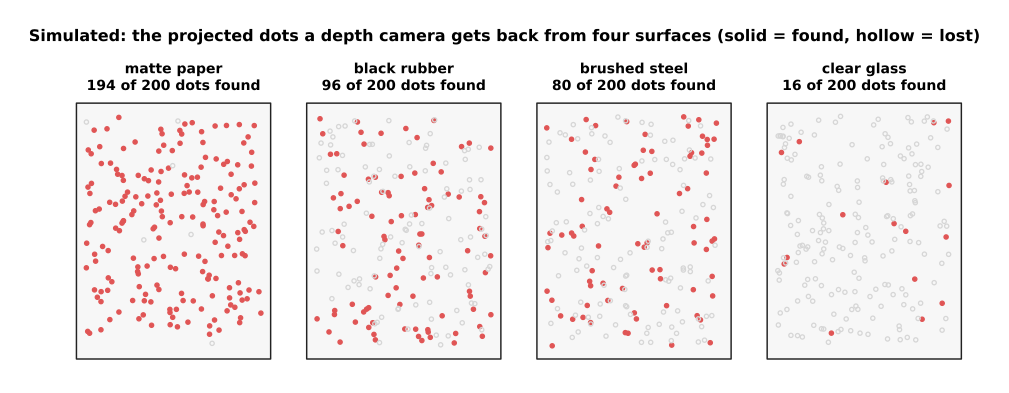
In this simulation matte paper returns 194 of 200 dots, black rubber returns 96, brushed steel returns 80 and clear glass returns only 16.
The three failures have three different causes. A dark surface absorbs the infrared light instead of scattering it back. A shiny surface sends the light off in one direction, and that direction is usually not back towards the camera. A clear surface lets the light through almost unchanged. The fractions above are invented, but the ordering is what happens in a workshop.
A dot that does not come back leaves a pixel with no distance in it, which is called a hole. The picture below shows a simulated depth map with four patches of different material in it, where black means the camera got no distance for that pixel.
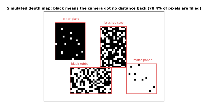
Over the simulated map 78.4 per cent of all pixels carry a distance, and the holes are concentrated inside the four patches.
The picture below counts the filled pixels inside each patch, so that the four materials can be compared directly.
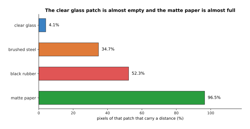
Only 4.1 per cent of the clear glass patch carries a distance, against 34.7 per cent for brushed steel, 52.3 for black rubber and 96.5 for matte paper.
A hole in a depth map is not the worst outcome, because a program can see that a pixel has no distance and refuse to act on it. The dangerous case is a wrong distance that looks exactly like a right one, and clear glass produces that case every time.
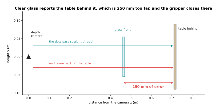
The glass stands at 0.460 metres and the table behind it at 0.710 metres, so the dots pass through the glass and come back off the table, and the camera reports the glass as 250 millimetres further away than it is.
A gripper sent to 0.710 metres travels 250 millimetres past the front of the glass before the fingers close. It therefore drives into the glass and knocks it over, and nothing in the depth map warned it. The usual answers are to find the transparent object in the colour picture and fill its depth in from a model trained for that job, or to feel for the surface with a force sensor instead of trusting the camera. The catalogue page on depth from pictures names the models built for transparent objects.
6. From a depth picture to a shape the arm can use#
Sections 2 to 5 all produced a depth map, and a depth map is still laid out as a picture, while an arm does not move in picture coordinates. Turning the map into positions is three lines of arithmetic that use four numbers measured once when the camera was calibrated. The picture below works one pixel through those three lines.
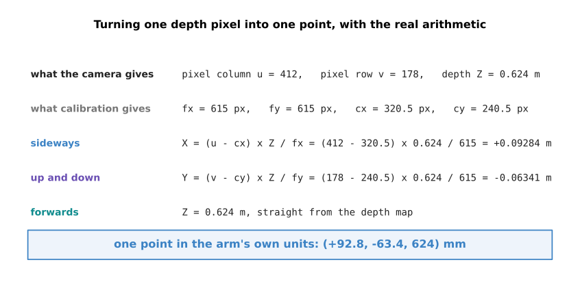
Pixel 412, 178 at a depth of 0.624 metres gives a sideways position of 0.09284 metres and an up-and-down position of -0.06341 metres, which is the point 92.8, -63.4, 624 in millimetres.
The sideways position is the pixel's column minus the column the lens looks straight through, multiplied by the depth and divided by the focal length. The up-and-down position is the same calculation with rows instead of columns. Doing that for every pixel that has a distance turns the map into the point cloud described on pictures, sound and robot states. The picture below draws a simulated table scene as such a cloud, from above and from the front.

The same cloud seen from above shows where the three objects sit on the table, and seen from the front shows how far each one stands up out of it.
A cloud like that is large. A 640 by 480 depth map has 307,200 pixels, and at the 78.4 per cent fill of section 5's simulated map that is 240,800 points. Three numbers a point at 4 bytes each is 2.9 megabytes for one frame, which is 87 megabytes a second at thirty frames a second.
A list of points also has one awkward property, which is that the order of its entries means nothing. The same tabletop can arrive as the same points in any order. A network that reads points must therefore give the same answer whatever order they come in, and an ordinary fully connected layer does not. The picture below sends five points through a small network, keeps the largest value in each column, and does it twice with the points in two different orders.
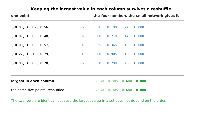
Keeping the largest value in each column gives 0.380, 0.905, 0.480 and 0.000 whatever order the five points arrive in, because the largest value in a set does not depend on the order of the set.
A layer that reads all fifteen numbers in one row behaves differently, and the picture below shows how differently.
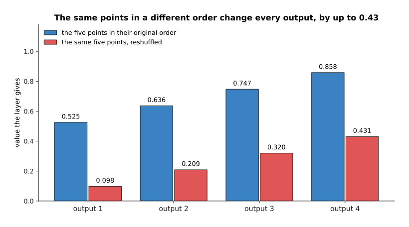
A layer that reads all fifteen numbers in one row changes every one of its four outputs when the same five points are reshuffled, by up to 0.43.
That is the whole trick behind networks that read points directly. Each point is treated on its own by a small network. The results are then combined by an operation that does not care about order, such as keeping the largest. Later layers look at each point together with its nearest neighbours, which is how such a network learns shape.
The alternative is to chop the space into equal cubes and record what falls in each cube. Each of those cubes is a voxel, which is the three-dimensional version of a pixel, and recording which cubes contain surface is called occupancy. The picture below takes one flat layer of such a grid and shades the cells that hold a point.
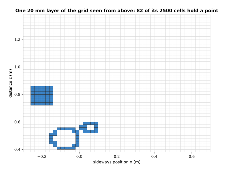
One 20 millimetre layer of the grid holds points in 82 of its 2,500 cells, and the rest of the layer is air.
Almost all of the grid is empty, and that is what decides how a voxel grid is stored. Over a one metre cube, a 5 millimetre grid has 8,000,000 cells, of which only 11,242 are touched by a point, which is 0.141 per cent. The picture below compares storing every cube against storing only the full ones, at three cube sizes.
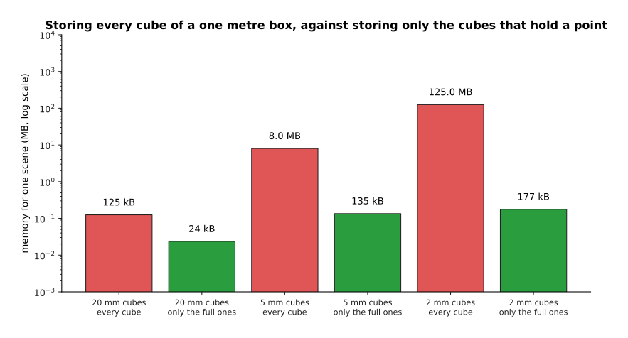
Storing every cube of a one metre box takes 8.0 megabytes at 5 millimetres and 125.0 megabytes at 2 millimetres, while a list of only the full cubes takes 135 and 177 kilobytes.
The appeal of a voxel grid is that it is regular, so the convolutions that work on pictures work on it unchanged. The cost is in that 0.141 per cent. Almost all of a room is air, which is why real systems store only the occupied cells, and why networks that read points directly are more common now.
7. Learned scenes: radiance fields and splatting#
Sections 1 to 6 all described one camera position at one moment, so a point cloud built that way has holes wherever the camera could not see. The last idea on this page is different in kind. Instead of measuring one view, it fits a description of the whole scene to many photographs at once, and then draws the scene again from any viewpoint you ask for.
The first way of doing this is a neural radiance field, which is a small network that answers one question. Given a place in the room and a direction you are looking from, the network says what colour is there and how solid it is. To draw one pixel you follow the ray out from the camera, ask the network at a series of points along that ray, and mix the answers in order so that a solid surface blocks what is behind it. The network is trained by drawing the photographs again and comparing them with the real ones. The picture below follows one such ray, and shows how much of the finished pixel each sample along it contributes.
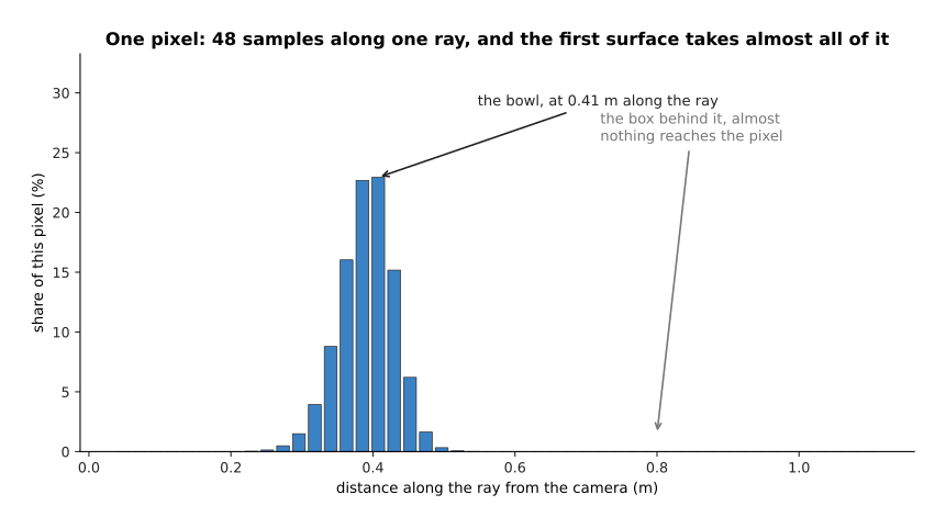
Along this ray the samples between 0.36 and 0.48 metres carry 84.7 per cent of the pixel between them, because that is where the bowl is, and the box standing behind the bowl contributes nothing at all.
That is a clean idea with an expensive consequence, because every sample on every ray is one call to the network. The picture below counts those calls for one picture.
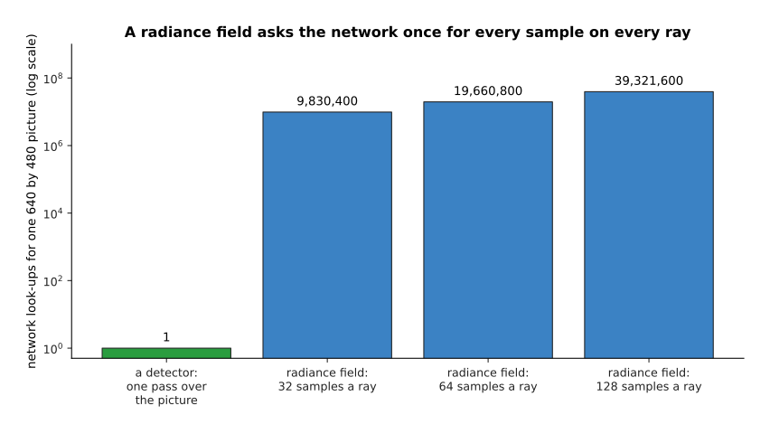
Drawing one 640 by 480 picture from a radiance field at 64 samples a ray takes 19,660,800 network calls, while a detector runs its network once over the whole picture.
Twenty million small network calls for one frame is why early radiance fields took many seconds to draw a single picture, which is far too slow for a robot that has to decide something now. Gaussian splatting solves the same problem by replacing the network with a pile of soft coloured blobs. Each blob stores a place, a width in each direction, a turn, a solidity, and a colour that varies with the direction you look from. Drawing the scene then means sorting the blobs by distance and painting them one over another, with no network call at all. The speed is paid for in memory, and the picture below counts the cost.
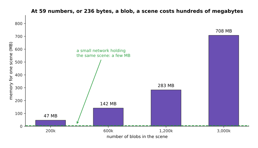
One blob keeps 3 numbers for where it is, 3 for its widths, 4 for its turn, 1 for its solidity and 48 for its colour, which is 59 numbers or 236 bytes, so 1.2 million blobs take 283 megabytes.
That is the honest trade. Splatting is fast enough to draw many times a second on an ordinary graphics card, which is what made this family of methods usable at all, and it pays for that speed in memory, because a scene is hundreds of megabytes rather than the few megabytes a small network takes. Both methods are also fitted to one scene rather than trained once and used everywhere. Moving the robot to a new room therefore means fitting a new scene from new photographs, which takes minutes. Methods that predict the blobs in one pass from a handful of photographs exist and are improving quickly, but a per-scene fit is still what most working systems do.
What a robot gets for that cost is a view it never took. The picture below shows an invented table scene as nine blobs seen from above, with the place a photo was taken from and a second place nobody stood at.
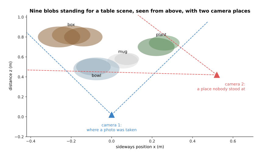
From the photographed place three of the nine blobs are visible, while from the second place six of them are.
The picture below draws what each of those two cameras sees. Each strip is 160 rays wide, and the red bar under each strip marks the rays the mug fills.
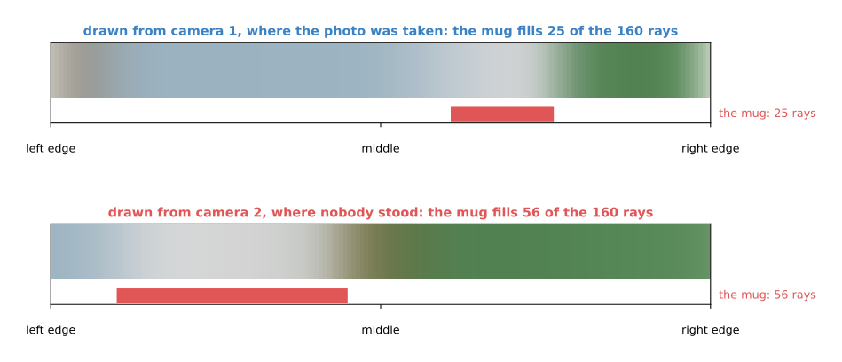
From the photographed place the mug fills 25 of the 160 rays, and from the place nobody stood at the mug fills 56, drawn from the same fitted scene.
Asking what the shelf looks like from above, without moving the camera there, is worth a great deal to a grasp planner. A grasp is chosen from a shape, and a shape built from one viewpoint is missing its back. The catalogue page on scene reconstruction lists the real systems of both kinds. In 2026 a depth camera is still what measures the table in front of the arm, while a fitted scene is what you build when you need the whole object or a view from somewhere the camera cannot go.
8. Where to read next#
- Recipes for models that see and understand gives the starting recipe for each of these: what one training example is, how many you need, what to begin from, and the mistake almost everybody makes first.
- Large language models is the next page, and it starts the chapter on models that read and write words rather than look at pictures.
- Pictures, sound and robot states explains how a point cloud is fed to a network as numbers, which is the step before section 6's layers.
- World models uses learned scene descriptions of the kind in section 7 to predict what happens next.
- Depth from pictures is the catalogue of the real single-picture and stereo depth models, including those built for transparent objects.
- Point cloud models is the catalogue for section 6's networks that read points directly, inside the wider 3D models chapter.
9. Using it in Python#
Section 6 turned one pixel into one point, and the code below does that for a whole depth map in NumPy. That is how it is done in practice, because NumPy does every pixel at once. The four lens numbers are the ones from section 6.
import numpy as np

fx, fy, cx, cy = 615.0, 615.0, 320.5, 240.5     # section 6's calibrated lens
depth = np.full((480, 640), 0.624)              # a depth map, in metres
depth[0, 0] = 0.0                               # a pixel with no distance

rows, cols = np.mgrid[0:depth.shape[0], 0:depth.shape[1]]
x = (cols - cx) * depth / fx                    # section 6: sideways
y = (rows - cy) * depth / fy                    # section 6: up and down
cloud = np.stack([x, y, depth], axis=-1)[depth > 0]   # drop the empty pixels

print(cloud.shape)                              # (307199, 3)
print(np.round(cloud[178 * 640 + 412 - 1], 5))  # [ 0.09284 -0.06341  0.624  ]

f, baseline, pixel_error = 700.0, 0.060, 0.25   # section 4's stereo pair
for z in (0.40, 1.00, 4.00):
    print(z, round(f * baseline / z, 1),        # disparity in pixels
          round(z ** 2 / (f * baseline) * pixel_error * 1000, 1))   # error in mm
The point printed for pixel 412, 178 is [0.09284 -0.06341 0.624], which is
section 6's worked example. The stereo loop then prints section 4's numbers:
105.0 pixels and 1.0 millimetres at 0.40 metres, 42.0 pixels and 6.0 millimetres
at 1 metre, and 10.5 pixels and 95.2 millimetres at 4 metres. One pixel is
dropped by the depth > 0 test, which is why 307,200 pixels give 307,199 points.
The libraries take over above that line. A depth camera's own driver gives you
the depth map and the four lens numbers already measured. The Open3D package
holds point clouds and does the filtering and plane-finding that section 6
implies. Hugging Face transformers loads a single-picture depth model with
pipeline('depth-estimation'), so that section 2's guess is one call. None of
them removes the arithmetic above, because every one of them expects you to know
whether your numbers are in metres.
What you still have to decide is which source of depth to use, and sections 2 to 5 are the list of trades. A single-picture model is free and gives relative depth, which section 3 showed is useless for reaching unless you pin it with measured anchors. A stereo pair measures real distances, and section 4 showed that its error grows with the square of the distance and that matching fails without texture. A pattern-throwing camera fixes the texture problem, and section 5 showed that it fails on glass in the worst possible way, by returning a confident wrong number. Most working arms use a pattern-throwing camera for the table, and reach for one of the others only where that camera is known to fail.