This page explains proportional-integral-derivative (PID) control, which is the standard way to make one joint of an arm go to a target angle and stay there. It answers four questions. What do the three parts of a PID controller each do, and how does a program run one, tick by tick? Where does a robot arm use it, and what goes wrong when it is set up badly?
It is written for a reader who has already read the overview
of this chapter, so you need to know what a joint angle and a motor are. But you do
not need any control theory or calculus, beyond knowing that a speed is how fast
something changes. Every number on this page comes from a real run of the diagram
script, docs/diagrams/control_and_motion.py, which simulates a joint rather than
drawing its curves by hand.
PID is the most used control technique in robotics, because it runs inside the drive of nearly every joint of nearly every arm, and inside most grippers, pan-tilt camera heads and conveyors too. This means it is usually the first thing to try, and it is often the last thing you need.
Contents#
- What this page answers
- The idea in one sentence
- How it works, step by step · The joint in the examples · P: push in proportion to the error · I: push harder while an error lasts · D: brake when the error is changing fast · A worked example: the first ticks by hand · The steps as pseudocode · Tuning the three gains · Two fixes every real PID needs
- Where it is used on a robot arm
- Where it is useful, and where it is not
- Libraries that provide it
- Why PID, and what it costs
- The learned alternative
- Where to read next
- Using it in Python
1. What this page answers#
A motor does not know anything about angles, because all it produces is a torque, a turning force measured in newton metres (N m), in proportion to the electric current sent to it. So if you want a joint at 30 degrees, something has to choose the torque, moment by moment, that gets it there.
That is harder than it sounds, because several things pull against the motor at once. Gravity pulls the link down, friction in the gearbox resists every movement, and the load in the gripper changes from one pick to the next. This means a torque worked out in advance for one case is wrong for the next case.
The answer is to measure and then correct, over and over. The joint's encoder is a sensor that reports the joint angle, so a controller can read it, compare it with the target, and choose a torque. Then it does the same again a millisecond later, and this repeating measure-and-correct cycle is called a feedback loop. PID is simply the rule that the loop uses to turn the error into a torque.
This page builds that rule one part at a time on a simulated joint, shows the numbers, and then shows the two faults that every real PID must be protected against.
2. The idea in one sentence#
Since the feedback loop needs a rule, here is the PID rule in one sentence. A PID controller sets the motor torque to the sum of three terms: one in proportion to the error now, one in proportion to the error added up over time, and one in proportion to how fast the error is changing.
Here is an everyday example of those same three terms, the cruise control in a car, where the driver sets a speed of 100 km/h.
- If the car is going 90 km/h, the controller presses the accelerator in proportion to the 10 km/h gap. That is the proportional part.
- On a long hill, a fixed press is not enough, and the car settles at 97 km/h. The controller notices that the gap has lasted a long time, and slowly presses harder until it is gone. That is the integral part.
- When the car is gaining speed quickly, the controller eases off a little before it reaches 100 km/h, so it does not shoot past. That is the derivative part.
A joint controller does exactly the same, with an angle instead of a speed and a motor torque instead of an accelerator pedal.
3. How it works, step by step#
The joint in the examples#
Because the three terms are easier to compare on one example, every picture on this page uses the same simulated joint, which has these properties:
- an inertia of 0.05 kg m². Inertia is how hard it is to start or stop the joint turning. It plays the part that mass plays in a straight line.
- friction of 0.5 N m for every radian per second of speed. A radian is the unit of angle a program uses; 1 radian is about 57.3 degrees.
- a steady pull of gravity of 1.0 N m on the link. The moves are small, so the pull is treated as constant.
- a controller that runs 1,000 times a second, a common rate for a joint loop. Each run is called a tick.
The task is the same in every picture: the joint rests at 0 and is told to go to 0.5 radians, about 29 degrees. A sudden change of target like this is called a step.
P: push in proportion to the error#
The first of the three terms is also the simplest one. The error is the target angle minus the measured angle, and the proportional term is that error times a number called the proportional gain, written Kp:
P = Kp × error
With Kp = 20 N m per radian, an error of 0.5 radians gives a torque of 10 N m, and as the joint gets closer the error shrinks, so the push shrinks with it.
The left panel below shows what P alone does.
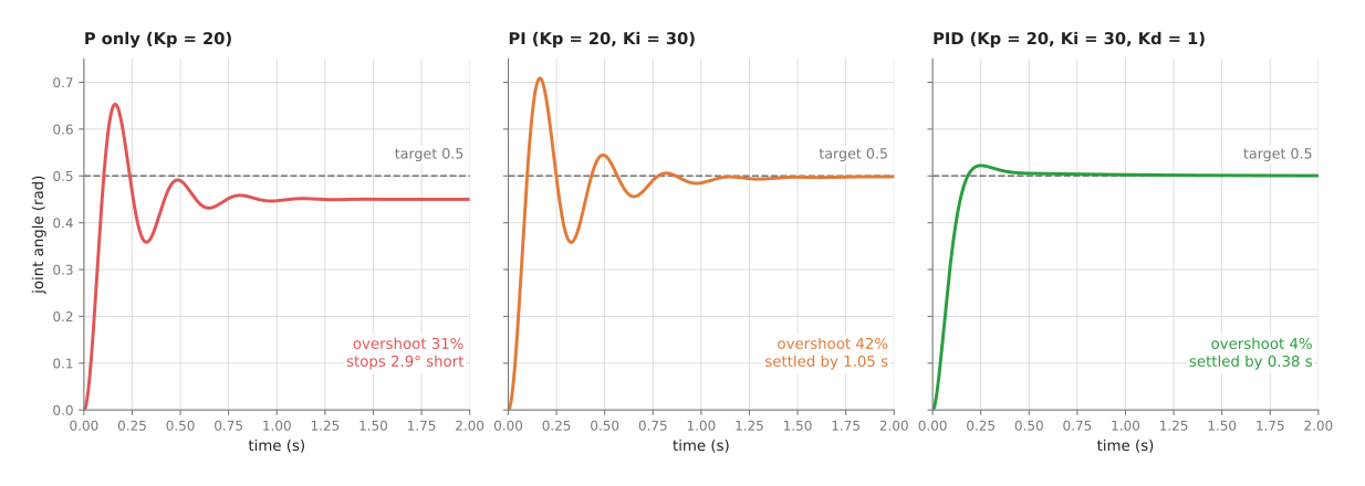
Each panel is one simulated run of the same step with different terms switched on, and the dashed line in each panel is the target.
P alone has two faults. First it overshoots, because the joint swings 31 per cent past the target before it turns back. Second it stops short, because it comes to rest 0.05 radians, or 2.9 degrees, below the target.
The overshoot happens because nothing slows the joint down on its way in. The torque only reaches zero at the target, so the joint arrives at full speed.
The stopping short is worth understanding, because it is the most common fault of a P controller. At rest the motor must hold up the link against gravity's 1.0 N m, but a P controller only produces torque when there is an error. So it must keep an error of 1.0 ÷ 20 = 0.05 radians just to hold the link up, and this leftover error is called the steady-state error. A larger Kp makes it smaller, but it never makes it zero, and a larger Kp also makes the overshoot worse.
I: push harder while an error lasts#
Because the P term leaves that steady-state error behind, a second term is needed to take it away. The integral term adds up the error over time, so on each tick it adds the error times the length of the tick to a running total. That total, times the integral gain Ki, is the integral term:
total = total + error × tick_length
I     = Ki × total
While any error remains the total keeps growing, and so does the push, and it only stops growing when the error is exactly zero. That is how the integral term removes the steady-state error, because it finds, by itself, the 1.0 N m that gravity needs.
The middle panel of the picture shows PI control, with Kp = 20 and Ki = 30, and the joint now ends on the target. But the overshoot is worse, at 42 per cent, and the joint rings for about a second before it settles. This happens because the integral term keeps pushing on the way in, since the total was built up while the joint was still short of the target.
D: brake when the error is changing fast#
Since the integral term made the overshoot worse, a third term is needed to take the overshoot away again. The derivative term looks at how fast the error is changing, which for a still target is the same as the joint's speed with the sign turned round. The term is that rate of change times the derivative gain Kd:
D = Kd × (rate of change of the error)
  = − Kd × (joint speed)      when the target is not moving
When the joint is rushing towards the target the error is shrinking fast, so D produces a large torque in the opposite direction, which works as a brake that is strongest when the joint is fastest.
The right panel of the picture shows full PID control, with Kp = 20, Ki = 30 and Kd = 1. As a result the overshoot drops to 4 per cent, and the joint is within 2 per cent of the target by 0.38 seconds and stays there.
The table below collects those three runs, so that they can be compared directly. Read each row as one controller, and read the columns as the overshoot, the time after which the joint stays within 2 per cent of the target, and the error left at the end of the 3-second run.
| Controller | Overshoot | Settled within 2 per cent by | Error at the end |
|---|---|---|---|
| P (Kp = 20) | 31 per cent | never | 0.050 rad (2.9 degrees) short |
| PI (Kp = 20, Ki = 30) | 42 per cent | 1.05 s | 0.0003 rad |
| PID (Kp = 20, Ki = 30, Kd = 1) | 4 per cent | 0.38 s | less than 0.0001 rad |
The picture below splits the PID run into its three terms, so you can see what each one does at each moment.
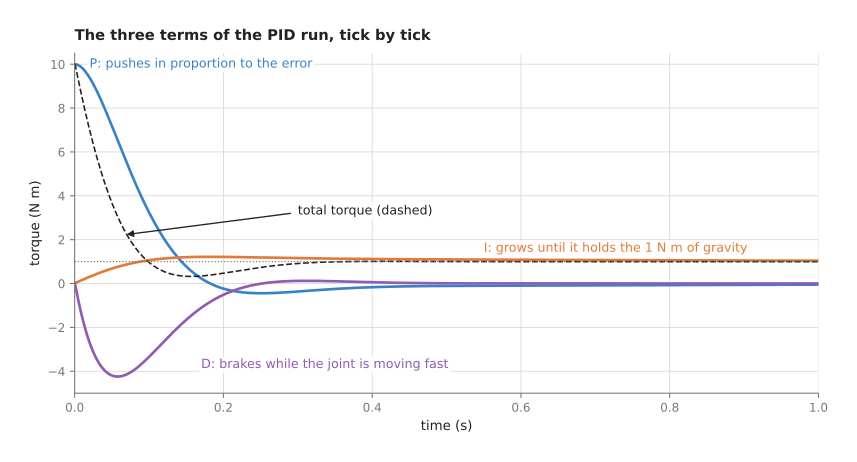
At the start the P term does almost all the work, because it alone gives 10 N m. Then the D term quickly goes strongly negative, down to about −4 N m, while the joint is moving fast, and that is the braking. Meanwhile the I term grows slowly and levels off at 1.0 N m, which is exactly the pull of gravity. Once the joint is at rest on the target, P and D are both zero, so the I term alone holds the link up. The dashed line is their sum, which is the torque actually sent to the motor.
One detail of this controller matters a great deal in practice, which is that it takes the rate of change of the measured angle rather than of the error. For a still target the two are the same. But when the target jumps the error jumps with it, and its rate of change for one tick is enormous. This means a controller that differentiates the error would send one huge kick of torque at every new target, so differentiating the measurement avoids that, and most library PID controllers offer it as an option.
A worked example: the first ticks by hand#
Since the three terms are easier to trust once you have seen them worked out, here are the first ticks of the PID run, with Kp = 20, Ki = 30, Kd = 1 and a tick of 0.001 s. The numbers all come from the simulation.
Tick 0, at time 0. The joint is at 0, so the error is 0.5.
- P = 20 × 0.5 = 10.0 N m.
- The total becomes 0 + 0.5 × 0.001 = 0.0005, so I = 30 × 0.0005 = 0.015 N m.
- The joint has not moved, so D = 0.
- The torque is 10.0 + 0.015 + 0 = 10.015 N m.
Tick 1, at 0.001 s. The torque has moved the joint to 0.0000989 radians.
- The error is 0.5 − 0.0000989 = 0.4999, so P = 9.998 N m.
- The total becomes 0.0005 + 0.4999 × 0.001 = 0.0009999, so I = 0.030 N m.
- The joint moved 0.0000989 radians in 0.001 s, a speed of 0.0989 radians per second, so D = −1 × 0.0989 = −0.099 N m.
- The torque is 9.998 + 0.030 − 0.099 = 9.929 N m.
By tick 100, at 0.1 s, the joint is at 0.338 radians and moving fast. P has fallen to 3.24 N m, I has grown to 1.07 N m, and D is −3.34 N m, braking hard. So the torque is 0.96 N m, which is less than gravity, and the joint is already slowing down.
At the end of the run, the I term is 1.0014 N m and the other two are almost zero.
The steps as pseudocode#
Once those three terms are clear, the whole controller is only a few lines, run once per tick. The pseudocode below uses plain names, so it works in any language.
set total = 0
set previous_measured = read_encoder()

every tick (tick_length seconds):
    measured = read_encoder()
    error    = target - measured

    p = Kp * error

    total = total + error * tick_length
    i = Ki * total

    speed = (measured - previous_measured) / tick_length
    d = -Kd * speed
    previous_measured = measured

    torque = p + i + d
    if torque > torque_limit:     torque = torque_limit
    if torque < -torque_limit:    torque = -torque_limit
    send torque to the motor
The last three lines clip the torque to what the motor can actually give, and the
two fixes in the section after next change the total line and the speed line.
Tuning the three gains#
Since the three gains decide how the loop behaves, choosing Kp, Ki and Kd has a name of its own: tuning. There are formal methods for it, but most arm joints are tuned by hand in this order.
- Set Ki and Kd to zero. Raise Kp until the joint reaches the target quickly and overshoots a little. It will stop short under load.
- Raise Kd until the overshoot is gone. Too much Kd makes the joint sluggish and noisy.
- Raise Ki until the steady-state error disappears in a reasonable time. Too much Ki brings back overshoot and ringing, as the PI panel shows.
- Test with the heaviest and lightest loads the arm will carry, and at the ends of its range, where gravity pulls hardest.
A well-known formal starting point is the Ziegler–Nichols method, where you raise Kp alone until the joint oscillates steadily, note that gain and the time of one swing, and read the three gains off a table. But the result is usually too aggressive for an arm, so treat it as a first guess rather than an answer.
A large improvement often comes from outside the three terms. If you know the pull of gravity at each angle, from the arm's mass model, you can add it to the torque directly. This is called gravity compensation, a kind of feed-forward, meaning a torque sent because you know it is needed rather than because an error was measured. This means the I term then has almost nothing left to do, so it can be kept small.
Two fixes every real PID needs#
The pseudocode above works in the simulation, because the simulation has a perfect encoder and an unlimited motor. But a real joint has neither of those, so two faults follow, and each one has a standard fix.
The first fault is integral windup, and it starts with the fact that a real motor has a torque limit. On a large move the controller asks for more than that limit, so the motor gives only the limit, and the joint moves more slowly than the controller expects. Because the error then stays large, the integral total keeps growing the whole time. So when the joint finally reaches the target the total is far too large, and the joint shoots past and takes a long time to come back.
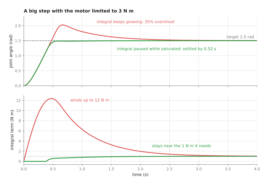
The picture shows a 1.5 radian step with the motor limited to 3 N m. In the red run the integral term grows to 12 N m while the motor is at its limit, which is twelve times the 1 N m it really needs. As a result the joint overshoots by 35 per cent and takes 2.36 seconds to settle. The fix, called anti-windup, is to stop adding to the total while the torque is being clipped. So in the green run the total is paused whenever the motor is at its limit, and the joint does not overshoot at all and settles by 0.52 seconds.
The second fault is derivative noise, and it comes from the encoder rather than from the motor. An encoder does not report a smooth angle, because it counts steps instead. A common encoder has 4,096 counts per turn, so one count is 0.0015 radians. This means that when the angle moves by one count between ticks, the measured speed jumps from 0 to 0.0015 ÷ 0.001 = 1.5 radians per second for one tick, and the D term turns that into a sudden spike of torque.
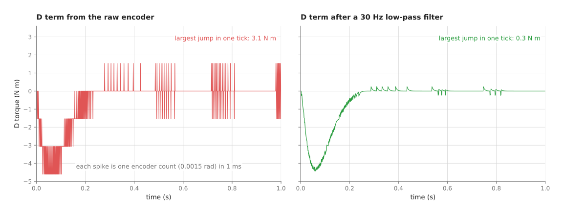
The left panel is the D term of the PID run with a 4,096-count encoder, and it is a train of spikes. The largest jump from one tick to the next is 3.1 N m, and after the first second, when the joint is almost still, the D term's typical size (its standard deviation) is still 0.81 N m. Because the motor turns those spikes into noise and heat, a fix is needed, and it is a low-pass filter, a small calculation that lets slow changes through and smooths away fast ones. The right panel filters the speed so that changes faster than about 30 times a second are damped. As a result the largest jump falls to 0.3 N m, and the typical size after the first second falls to 0.09 N m, while the step response hardly changes: the overshoot goes from 4.4 per cent to 3.1 per cent.
But a filter delays the signal a little, and too much delay makes the loop unstable, so the filter is set as slow as the noise requires and no slower. A Kalman filter is a more careful way to get a clean speed from a noisy angle.
4. Where it is used on a robot arm#
Because PID is used anywhere that a measured number must be held at a target, on and around an arm that means almost everywhere.
The joint position loop. This is the main use, because each joint's drive runs a PID loop on the joint angle. In many drives it is the outer loop of three: a position loop chooses a speed, a speed loop chooses a current, and a current loop, often running 10,000 or more times a second, sets the motor current. Each of the three is a PID or a PI loop, so when an arm maker says "position-controlled arm", this cascade is what is inside.
Following a trajectory. The target does not have to be still, because the trajectory generation page produces a new target for every tick, and the same PID loop follows it. That is why the lag in the overview's move appears, since it is a PID loop following a moving target. Adding the trajectory's own speed and acceleration as feed-forward shrinks that lag a great deal.
Gripper fingers. An electric gripper runs a position loop on its finger gap, with the current limited so that the squeeze is limited. The Book 3 page on holding on explains why that current limit is not the same as a force setting.
Pointing a camera. A pan-tilt head, or a wrist camera centred on an object, can be steered by a PID loop whose error is measured in pixels: how far the object is from the middle of the picture. This is the simplest form of visual servoing, described in controlling the move. It is usually P or PI only, because the camera is slow and noisy.
Holding a force. An admittance controller, explained on the impedance and force control page, can include a PI loop on the force error. Its target is a force, such as "press with 10 N", and its output is a small change of position.
Conveyors and turntables. A conveyor that must match the arm's pick timing, or a turntable that presents parts, is held at speed by a PI loop.
5. Where it is useful, and where it is not#
The uses above all share the same conditions, because PID works best when the thing being controlled responds in a simple, steady way, the sensor is fast and clean, and the target changes smoothly. So it struggles as soon as any one of those is false.
The table below lists the common failures. Read each row as one situation, giving the sign you would see on the arm or in the logged data, and what people use instead or add to fix it.
| Situation | The sign you would see | What people use instead or add |
|---|---|---|
| The load changes a lot, such as an empty gripper against a 3 kg part | good tuning with one load, overshoot or sagging with the other | gravity compensation from a mass model; gains scheduled by load; a learned arm model as feed-forward |
| Fast moves on a heavy arm, where joints push on each other | following error that grows with speed and changes with pose | computed-torque control from a dynamics model, such as Pinocchio's; PID remains on top to clean up |
| A slow or delayed sensor, such as a camera at 30 frames a second | the arm oscillates around the target, more with higher gain | lower gains; model predictive control; a Kalman filter that predicts across the delay |
| The motor hits its torque limit | a large overshoot after big moves only | anti-windup, as shown above |
| A noisy sensor | a buzzing or hot motor, spiky torque traces | filter the D term, or drop it and use PI |
| Friction that sticks and then lets go, common in gearboxes | the joint stops just short, then jumps past, and repeats slowly | friction compensation; a small dead band around the target |
| Contact with a rigid surface | the force climbs to the motor's limit | impedance or force control, not a better PID |
| Several goals at once, such as speed limits and staying inside a region | limits broken, or clipping that ruins the tuning | model predictive control, described in controlling the move |
The row about contact is the most important one in that table. A PID position loop is doing its job correctly when it pushes harder into a table it cannot pass through, so no amount of tuning fixes that, because pushing until the error is gone is exactly what the loop is for. The impedance and force control page shows the force climbing to the motor's limit in a simulation.
6. Libraries that provide it#
Since the loop is short enough to write yourself, many people do, but the libraries below include the anti-windup, filtering and tuning helpers that are easy to get wrong. The table lists the well-known ones. Read each row as one library, giving the languages it is used from, the class or function, and a note on what it is for.
| Library | Languages | Class or function | Note |
|---|---|---|---|
| ros2_controllers | C++, configured from YAML | pid_controller; joint_trajectory_controller gains | pid_controller runs a PID on any command interface; the trajectory controller uses per-joint PID gains when it commands velocity or effort instead of position |
| control_toolbox (ros-controls) | C++ | control_toolbox::Pid | the PID class used inside ros2_controllers, with integral clamping |
| simple-pid | Python | simple_pid.PID | a small pure-Python PID with output limits and anti-windup, good for scripts and tests |
| python-control | Python | control.tf, control.step_response | for trying gains on a model of the joint offline, before touching the arm |
| Gazebo (gz-math) | C++ | gz::math::PID | the PID used by Gazebo's joint controller plugins |
| MuJoCo | C, Python, XML model files | the position actuator, with its kp gain | a P controller with a damping option, built into the simulated actuator |
| Pinocchio | C++, Python | computeGeneralizedGravity, rnea | not a PID; computes the gravity and dynamics torques used as feed-forward alongside one |
On a real arm you usually do not write the joint loop at all, because it runs inside the arm maker's drive, and you tune it only through their software, if at all. So the PIDs you write yourself are the outer ones: a gripper, a camera head, a force loop, or a joint on a robot you built.
7. Why PID, and what it costs#
To put all of the above together, PID is a rule that sets a motor's output from the error now, the error summed over time, and the error's rate of change. This means it gives each joint the ability to reach a target and hold it against gravity, friction and changing loads, using only its own sensor and three numbers.
The first obvious alternative is to use no feedback at all, meaning that you work out the torque from a model of the arm and simply send it. That is called open-loop control, and it needs no sensor and cannot oscillate. But any error in the model, a change of load, or a knock from outside is never corrected, because nothing measures it. Even the simple joint on this page shows the problem, since a torque that is 10 per cent too small to hold up the link does not leave it a little short, it lets it fall. So feedback is chosen because the real arm never matches the model.
The second obvious alternative is a controller built on a full model of the arm's dynamics, such as computed-torque control or model predictive control. These use the arm's masses and inertias to work out the torque for the whole move, and can follow fast moves far more closely. But they need an accurate model, which means measuring the inertias of every link, and they are much harder to write, check and debug. PID needs no model at all, and its three numbers can be tuned by hand in an afternoon. That is why the usual practice is to add a model's torque on top of a PID loop rather than replace it.
The costs are these. You must tune three numbers, and the right values change with the load and the pose, while some error always remains for as long as the joint is moving. The integral term needs anti-windup and the derivative term needs a filter, or the loop misbehaves on a real motor. And a PID position loop has no idea of contact, so it will push as hard as the motor allows to reach a target inside a solid object.
8. The learned alternative#
Because the loop must answer every few milliseconds, there is no learned model that replaces it, since a network is almost never fast enough to sit inside such a loop. Book 7's running a model on a robot explains the usual split: a learned policy runs at its own slower speed and gives targets, and a fast programmed loop such as PID follows them. A learned arm model helps the loop instead of replacing it. It learns the torque each joint needs, including gearbox friction and cable pull that the textbook model leaves out, and that torque is added to the PID output as feed-forward. This pays off when wear or a new gripper makes plain PID lag, and the size of the learned correction should be limited, because a learned model gives no guarantee. Learning can also pick the gains themselves: Book 7's Bayesian optimisation tries a few sets of gains on the real joint, scores each test move, and chooses the next set to try, so it finds good gains in tens of trials instead of hand tuning.
9. Where to read next#
- The next page is trajectory generation. It makes the smooth, moving targets that a PID loop follows, instead of sudden steps.
- Impedance and force control changes what the loop does on contact.
- The Kalman filter gives a cleaner angle and speed to feed into the loop.
- Book 3's controlling the move shows the ROS 2 controllers that contain these loops, and the tolerances that decide whether a move "succeeded".
10. Using it in Python#
Section 3 built the loop term by term and ended with the two fixes that every real PID needs, which are the integral clamp and the filtered derivative. Section 6 then named the libraries that already contain those two fixes. This section shows the shortest honest Python that runs a PID, so that you can see how little of it the library covers and how much of it stays yours.
The example uses simple_pid, because it is pure Python and installs with one
command, which makes it the easiest way to try gains on a gripper or a camera head.
from simple_pid import PID

pid = PID(Kp=8.0, Ki=2.0, Kd=0.5,
          setpoint=1.0,                 # the angle we want, in radians
          output_limits=(-4.0, 4.0))    # the joint's torque limit, in newton metres
pid.sample_time = None                  # this loop decides when to tick, not the library

while running:
    torque = pid(read_joint_angle(), dt=0.002)   # one tick of a 500 Hz loop
    send_joint_torque(torque)
    log(pid.components)                 # the P, I and D parts of this tick, for tuning
That is the whole call. What the library does for you is the bookkeeping that is easy
to get wrong. It keeps the running sum for the integral term and clamps that sum to
output_limits, so the integral cannot keep growing while the motor is already at
full torque, which is the windup described in section 3. It clamps the output to the
same limits. It also takes the derivative of the measurement rather than of the error,
because differential_on_measurement is true by default, so moving the setpoint no
longer produces the sudden kick that a plain derivative of the error would give.
Finally pid.components hands you the three terms separately, which is what you look
at while tuning.
What you still write is everything that touches the arm. read_joint_angle and
send_joint_torque are your functions, because they depend on your driver. The loop
itself is yours, and it has to run at a steady rate, because the library does not
provide a timer. Setting setpoint on every tick from a trajectory generator is
yours, and so is deciding what to do when the loop cannot keep up. If several joints
move together you create one PID object per joint, as the
chapter overview does, because one object
holds the history of one signal only.
What you have to decide or measure is the short list that actually determines
behaviour. The three gains Kp, Ki and Kd come from tuning on the real joint by
the method in section 3, and copying them from another arm does not work because they
depend on that joint's mass and friction. The output limits come from the motor's data
sheet, in the same unit that your driver expects, and getting that unit wrong is a
common and dangerous mistake. The dt you pass has to be the period you really
achieve, not the one you hoped for. Finally the sign convention is yours to check: if
a positive torque turns the joint the other way on your arm, a correctly tuned PID
will drive it away from the target instead of towards it.