This chapter is about turning a planned path into smooth, safe motor commands. It covers five techniques: proportional-integral-derivative (PID) control, trajectory generation, arm dynamics, safety monitoring, and impedance and force control. All five are written sets of rules that a program follows many times a second. That means none of them is trained from data.
This page is the overview of the chapter, and it answers four questions. What job do these techniques do for an arm, and what does each of the five do in one line? How do they work together on one real move, and how does this chapter connect to the rest of the book and to the learned movement models in Book 6?
It is written for a reader who knows what a joint, a joint angle and a motor are,
at the level of Book 1's arm overview.
It also helps to have read the planning and search overview,
because this chapter starts where that one stops, though you do not need any
control theory beforehand. Every number on these pages comes from a real run of a
diagram script, such as docs/diagrams/control_and_motion.py, which simulates a
joint, a move and a contact rather than drawing them by hand, while the arm
dynamics page uses docs/diagrams/control_and_motion_2.py, which simulates a
two-joint arm.
Contents#
- What control and motion is for
- Three layers, three questions
- The five techniques
- The five side by side
- How they work together on one move
- Loops that run at different rates
- How this chapter connects to the others
- Where to read next
- Using it in Python
1. What control and motion is for#
The book's map of techniques describes this category in one line: turning a planned path into smooth, safe motor commands.
Here is that same job in everyday terms, where you carry a full mug of coffee from the kitchen to a desk. Since you already know the route, what is left is how you walk it. You do not start at full speed, because the coffee would slop, and you do not stop dead at the desk for the same reason. While you walk, you keep correcting your hand, because the mug is never quite where you meant it to be. Then when you put the mug down, you lower it until you feel the desk, and only then do you stop pushing.
Because an arm carrying a mug faces the same problem, it has the same three jobs every time it moves.
- It must decide how fast to go along the route at each moment, without going faster, or speeding up faster, than the motors allow.
- It must make each motor actually follow that plan, even though gravity, friction and the load all push the joint off course.
- It must behave sensibly when it touches something. A mug put down on a table, a peg pushed into a hole, and a person bumping the arm all need the arm to give way a little instead of pushing harder.
The planner from the planning and search chapter does none of those three jobs, because all it hands over is a list of joint angles to pass through. That means it says where to pass but not when, and it knows nothing at all about motors or contact.
2. Three layers, three questions#
Because those three jobs are so different from one another, the work is split into layers, where each layer answers one question and hands its answer to the layer below it.
The trajectory layer answers "where should each joint be at each instant?", and a trajectory is simply a path with times attached to it. Since the same path can be driven slowly or quickly, and with gentle or sudden changes of speed, this is the layer that chooses which of those it will be.
The controller layer answers "what torque should each motor produce right now, so that the joint is where the trajectory says?", where a torque is a turning force measured in newton metres (N m). Then the controller reads the joint's sensor, compares the reading with the target, and chooses a torque, and it does this again and again, often 1,000 times a second. This repeated correction is called a feedback loop, because the measurement is fed back into the next decision.
The controller does that job better when it knows the arm's own body, and the arm's dynamics are what describe that body. That means they say how much torque each joint needs to hold the arm up against gravity and to speed it up. Because a controller can add that torque before any error appears, it follows fast moves far more closely than one that waits for an error to show up first.
The contact layer answers "what should happen when the arm touches something?". But a plain position controller has only one answer, which is to push harder until the joint is where it was told to be. Instead of that, the contact layer lets you choose the behaviour, such as "act like a soft spring" or "stop when the force passes 1 newton".
Beside all three layers runs a safety monitor, which does not command the arm itself. Instead it watches the commands and the measurements, and it stops the arm when a speed, a force, a position or a distance to a person goes outside its limit, or when a loop stops sending commands.
The Book 3 page on controlling the move describes these same layers in ROS 2, where they appear as the ros2_control framework and its controllers. While that page shows how to use them, this chapter explains the techniques inside them.
3. The five techniques#
Each page in this chapter explains one of those layers in depth, and the pages are split into two groups by how often you will meet them. The most used group holds the four techniques that run on nearly every arm, every time it moves: PID control, trajectory generation, arm dynamics and safety monitoring. Even an arm that only moves between fixed poses uses all four, although the dynamics and the safety checks are often hidden inside the arm maker's controller. The also used group holds impedance and force control, which is used often, but only in tasks where the arm touches things on purpose, such as pressing, inserting or being guided by hand. It also needs an arm or a sensor that supports it, which not every arm does.
Here is each technique in a line or two, and the first four of them make up the most used group.
- PID control makes one joint follow its target. It adds up three pushes: one in proportion to the error now, one that grows while an error lasts, and one that brakes when the error is changing fast. It is the loop that runs inside nearly every joint of nearly every arm.
- Trajectory generation decides where each joint should be at each instant. It turns a list of waypoints into smooth curves, and gives them a speed profile that keeps within the motors' limits of speed, acceleration and jerk.
- Arm dynamics works out the torque each joint needs: inertia times acceleration, plus the pull of gravity, plus a part that grows with speed. It holds the arm still with no error, lets a controller follow fast moves closely, and lets a simulator predict how the arm will move.
- Safety monitoring watches the arm's software limits: joint positions, speeds, torques, forces and the distance to people. A watchdog, a timer that every new command must reset, stops the arm when a loop stops sending commands. Speed and separation monitoring slows the arm as a person comes closer, and stops it if they come too close.
Then comes the remaining technique, which is the one in the also used group.
- Impedance and force control decides how the arm behaves in contact. It makes the arm act like a spring with a stiffness you chose, stops a move when a force sensor fires, and keeps contact forces inside a limit.
4. The five side by side#
Since each of the five techniques has now been described in a line, the table below sets them side by side. Read each row as one technique, and read the columns as what goes in, what comes out, how often it runs, and the sign that tells you the technique is set up badly.
| Technique | What goes in | What comes out | How often it runs | The sign of a bad setup |
|---|---|---|---|---|
| PID control | the target angle and the measured angle | a torque or a motor current | 1,000 times a second or more | the joint overshoots and rings, or stops a little short of the target |
| Trajectory generation | waypoints and the joint limits | a target angle for every tick of the controller | once per move, then read out at the controller's rate | the arm jerks at the start and end, or the tool wobbles after it stops |
| Arm dynamics | the joint angles, speeds and wanted accelerations, and the arm's masses | a torque for each joint, or the accelerations that a torque will cause | 1,000 times a second inside the controller; also inside every simulator | the arm sags when held still, lags on fast moves, or sets off false collision alarms after a grasp |
| Safety monitoring | the commands, the measured angles, speeds and forces, and the distance to people | carry on, slow down, or stop | every controller tick, 500 to 1,000 times a second | the arm stops for no reason, or does not stop when a limit is broken |
| Impedance and force control | the target pose and the measured force or position | a force or torque, or a changed target position | 500 to 1,000 times a second | the arm pushes too hard on contact, bounces off, or buzzes against a hard surface |
5. How they work together on one move#
The layers above are easier to follow on one real move of two joints, which the diagram script simulates. Once the planner has given four waypoints in the space of joint angles, the trajectory layer draws a smooth curve through them and gives it times. After that the controller layer drives each joint along the curve, using the PID controller from the PID page.
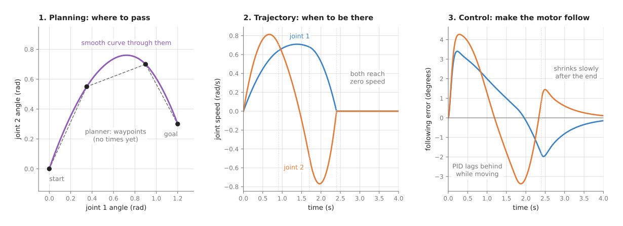
The left panel is the planner's output, together with the curve that the trajectory layer draws through it. The middle panel is the timing, meaning the speed of each joint over the 2.4 seconds of the move, while the right panel is the error of each joint, which is the target angle minus the measured angle.
Because each one shows a different layer doing its own job, three things in that picture are worth reading closely.
First, the planner's waypoints have no times of their own, so the trajectory layer is what chose them. In this run it gave each stretch of the path a share of the 2.4 seconds in proportion to its length, so the waypoints are passed at 0, 0.91, 1.70 and 2.40 seconds, and both joints start and end at zero speed.
Second, the controller never follows the trajectory exactly, because it lags behind while the joint is moving. The largest error is 3.4 degrees on joint 1 and 4.3 degrees on joint 2. This lag is called the following error, and it is perfectly normal. That is why the Book 3 page warns that a controller with its tolerances set to zero never checks it; see what "the move failed" actually means.
Third, the error is still not zero when the trajectory ends. At 2.4 seconds joint 1 is still 1.85 degrees off, and half a second later it is still 0.96 degrees off. This happens because the controller keeps working after the trajectory has stopped changing, and it closes the remaining gap slowly. That is why a move that is "done" by the clock is not always done at the joint, and the Book 3 page on the cost of a move calls this settling time.
This move has no contact in it, so the contact layer never runs. However, if the gripper were lowering a mug onto a table, the last few millimetres would be handed to that layer, as the impedance and force control page shows.
6. Loops that run at different rates#
The move above hid one thing, which is that the three layers do not run at the same speed. A planner runs once per move and may take a tenth of a second or more, while a controller runs every millisecond. But some sources of targets sit in between those two: a camera-based loop may send a new target 30 times a second, and a learned policy from Book 6 often sends one 10 to 15 times a second.
Because of that gap, something has to fill it between a slow stream of targets and a fast controller. The picture below shows why that matters, by sending the same 10 targets a second to the same joint in two different ways.
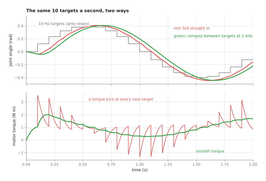
The red run sends each target straight to the controller and holds it there for 100 milliseconds, while the green run moves the target smoothly, 1,000 times a second, from the previous value to the newest one.
Because every new target in the red run is a small step, the controller answers each step with a sudden rise in torque. As a result, the largest change from one millisecond to the next is 2.48 N m, and the arm moves in small jerks. In the green run, however, the largest change in one millisecond is only 0.03 N m. But the green run has a cost of its own, because it is always one target behind, a tenth of a second late. The Book 3 page on learned motion describes exactly this trade, and it is the reason learned policies still need the trajectory and controller layers underneath them.
The general rule that follows from this is simple: every loop should hand the loop below it a signal that changes smoothly at the lower loop's own rate. The trajectory generation page shows how to build such a signal.
7. How this chapter connects to the others#
Because everything above turns a decision that has already been made into motor commands, control and motion sits at the end of the chain. The techniques in the other chapters decide what to do and where to go, and this chapter is what makes it actually happen.
- Planning and search hands over the path. Trajectory optimisation can already give a path with times, and then the trajectory layer here only checks and smooths it. Numerical inverse kinematics turns a target pose for the gripper into joint angles, which is also how a Cartesian controller works inside.
- Fitting and estimation cleans up the signals the controllers read. A Kalman filter can smooth a noisy joint speed or a noisy force reading before a controller uses it.
- Geometry and cameras provides the frames that a Cartesian impedance controller works in. The stiffness "along the tool" only means something once the tool frame is known.
- Decisions and task logic decides when to switch layers: for example, move fast in free space, then switch to a guarded move for the last 30 millimetres, then switch to impedance control to press.
Book 6 has learned models that do parts of this job as well. For example, a movement model decides where the arm should go next, from camera pictures, so it replaces the planner and sometimes the trajectory layer, but not the controller: its output is still a stream of joint targets that a PID loop must follow. A learned arm model predicts the torque a joint needs, and it usually corrects the physics model from the arm dynamics page rather than replacing it, so that the result can be added to a PID loop to make it follow more closely. A force and slip model reads the touch signals that a force controller could then act on. None of these removes the need for the programmed loops on this chapter's pages, because they sit on top of those loops rather than in place of them.
8. Where to read next#
- Start with PID control, because it is the loop inside every joint and the other pages all build on it.
- Then read trajectory generation, which makes the targets that PID follows.
- Then read arm dynamics, which adds the torque a PID loop would otherwise have to wait for an error to find.
- Then read safety monitoring, which watches all the other loops and stops the arm when a limit is broken.
- Then read impedance and force control, which changes what happens at contact.
- Book 3's controlling the move shows these layers in ROS 2, with the settings that ship with them.
- Book 3's holding on covers impedance and admittance from the gripper's point of view.
- Book 7's movement models overview shows what a learned policy takes over, and what it still leaves to these loops.
9. Using it in Python#
Section 5 followed one move through all five techniques, and section 6 showed that they run at different rates. This section puts the same stack into Python, so that you can see which library covers which layer and how the layers hand values to each other. After reading it you will know what a running control loop imports, and you will see that most of the lines in it are still yours.
The loop below moves a two-joint arm to a new pair of angles. Ruckig makes the moving target, Pinocchio works out the torque that target needs, and one PID per joint corrects whatever is left over.
import numpy as np, pinocchio as pin
from ruckig import InputParameter, OutputParameter, Result, Ruckig
from simple_pid import PID

DT = 0.002                                     # one tick every 2 milliseconds
model = pin.buildModelFromUrdf("arm.urdf")     # your arm's masses and lengths
data = model.createData()

otg = Ruckig(model.nq, DT)                     # layer 1: trajectory generation
inp, out = InputParameter(model.nq), OutputParameter(model.nq)
inp.current_position = [0.0, 0.0]
inp.target_position = [0.6, -0.4]
inp.max_velocity = [1.5, 1.5]
inp.max_acceleration = [3.0, 3.0]
inp.max_jerk = [20.0, 20.0]

pids = [PID(Kp=40.0, Ki=5.0, Kd=2.0, output_limits=(-30.0, 30.0))
        for _ in range(model.nq)]              # layer 3: one PID per joint
for p in pids:
    p.sample_time = None                       # the loop decides when to tick

while otg.update(inp, out) == Result.Working:
    q_d = np.array(out.new_position)           # where each joint should be on this tick
    # layer 2: the torque this motion needs, worked out before any error appears
    tau_ff = pin.rnea(model, data, q_d,
                      np.array(out.new_velocity), np.array(out.new_acceleration))
    q = read_joint_angles()
    for j in range(model.nq):
        pids[j].setpoint = q_d[j]
    tau_fb = np.array([pids[j](q[j], dt=DT) for j in range(model.nq)])
    send_joint_torques(clamp_to_limits(tau_ff + tau_fb))   # layer 4: safety monitoring
    out.pass_to_input(inp)                     # this tick's end state starts the next one
Three libraries appear there, and each one covers exactly one layer. Ruckig turns a
target angle into a jerk-limited position, speed and acceleration for every tick, and
it does that from whatever state the arm is in, which is the part of trajectory
generation that is hard to write correctly. Pinocchio reads the arm description and
computes the torque that the wanted acceleration needs, so you never write the
equations of motion yourself. simple_pid keeps the error history, clamps the
integral term so it cannot grow while the output is saturated, and clamps the output
to the limits you gave it.
Everything else in that loop is yours. read_joint_angles, send_joint_torques and
clamp_to_limits are your code, because they depend on which arm and which driver
you use, and no library can guess them. You also have to run the loop at a steady
rate, decide what happens when one tick arrives late, and put a state machine around
the whole thing so that a move can be started, paused and abandoned.
The numbers are yours too, and they are the part that decides whether the arm moves
well. The speed and acceleration limits come from the arm's manual, but the jerk
limit is usually in no manual, so you lower it until the wobble described in section
5 disappears. The three PID gains come from tuning on the real joint. The masses,
centres of mass and inertias in arm.urdf come from the arm maker if it publishes
them, and from your own measurements if it does not, and a held object is not in that
file until you add it. Finally DT has to match the rate your program really
achieves, because a PID tuned at 500 ticks a second behaves differently at 100.
One caution before you try this. On most industrial arms you cannot send torques at all, because the joint loop runs inside the maker's drive, as the PID page explains. In that case only layer 1 stays in your program, and you send positions instead of torques.