This page explains arm dynamics, which is how the torques at an arm's joints and the arm's motion are tied together. It answers five questions. What torque does each joint need to make a given move, and what happens to the arm when you send it a given torque? How does a controller use those answers to hold the arm still and to follow fast moves closely? And what changes when the gripper picks up a load, and how do you find out how heavy the parts of your own arm are?
It is written for a reader who has already read the page on
PID control. That page explains torque, error, feedback and
feed-forward on a single joint, and it mentions gravity compensation in one
paragraph. So this page takes that paragraph and builds it out for a whole arm. You
do not need any mechanics beyond knowing that a heavier thing is harder to speed up.
Every number on this page comes from a real run of the diagram script,
docs/diagrams/control_and_motion_2.py, which simulates a two-joint arm rather than
drawing its curves by hand.
Dynamics is one of the most used techniques in arm software, even though most users never see it. Instead it runs inside the drives of every torque-controlled arm, inside every arm simulator, and inside the collision detectors that stop an arm when it bumps a person.
Contents#
- What this page answers
- The idea in one sentence
- How it works, step by step · The arm in the examples · The three parts of a joint torque · A worked example: one instant by hand · Inverse and forward dynamics · Gravity compensation: holding still with no error · Feed-forward plus PID, and computed-torque control · A payload changes the numbers · Finding the arm's masses · The steps as pseudocode
- Where it is used on a robot arm
- Where it is useful, and where it is not
- Libraries that provide it
- Why a dynamics model, and what it costs
- The learned alternative
- Where to read next
- Using it in Python
1. What this page answers#
The PID control page drives one joint that has a fixed inertia and a fixed pull of gravity, but a real arm is not like that. The pull of gravity on the shoulder depends on how far out the rest of the arm reaches. In the same way, the effort needed to speed up the shoulder depends on whether the elbow is bent or straight. On top of that, when one joint swings fast it pushes and pulls on the others.
A PID loop can still cope, because it corrects whatever error it measures. But it only corrects an error after that error has appeared, so on a fast move the arm always lags behind. That is why the PID page's table of failures points to a torque worked out from a model of the arm's dynamics.
This page is about that model. The dynamics of an arm are the rules that link the forces on it to the way it moves. So once you have them, you can work out most of the torque each motor will need before the arm moves at all. This means the feedback loop then only has to clean up the small part that the model got wrong.
2. The idea in one sentence#
Since the model has to cover gravity, inertia and the push between joints, here it is in one sentence. The torque each joint needs is the sum of three parts: the arm's inertia times the acceleration you want, the pull of gravity on the arm in its current pose, and a part that depends on how fast the joints are already turning.
Here is an everyday example of those three parts, carrying a full shopping bag at arm's length. Just holding the bag still takes effort, and more effort the further out your arm reaches, and that is the gravity part. Swinging the bag up quickly takes extra effort at the start of the swing, and you must hold back at the end to stop it. That is the inertia part. And if you spin round on the spot while holding the bag, you feel it pull outwards even though you are not trying to move your arm at all, and that is the speed part.
A robot arm's software does exactly the same sums. It knows from the arm's description how heavy each link is and where its weight sits. So from that it works out all three parts, for every joint, a thousand times a second.
3. How it works, step by step#
The arm in the examples#
Because the three parts are easier to compare on one example, every picture on this page uses the same arm. It has the same shape as the book's two-link arm from Book 1's arm overview. But it is scaled down to the size of a real table-top arm, and it swings in a vertical plane, so that gravity pulls on it.
- Link 1, from the shoulder to the elbow, is 0.30 m long and weighs 2.0 kg.
- Link 2, from the elbow to the tip, is 0.25 m long and weighs 1.0 kg.
- Each link is a plain rod, so its weight is centred at its middle. The point where a link's weight is centred is called its centre of mass.
- Angles are measured from the horizontal. Joint 1's angle, q1, is the angle of link 1. Joint 2's angle, q2, is the bend at the elbow, measured from link 1.
- The real arm has a little friction in each joint, 0.02 N m for every radian per second of speed. The controllers' model of the arm believes it is 0.016, which is 20 per cent too low, because a measured friction value is never exact.
- The controllers run 1,000 times a second, as on the PID page.
The three parts of a joint torque#
Once that arm is fixed, the torque its two joints need can be written as one line:
torque = M(q) × acceleration + c(q, speed) + g(q)
Here q stands for the two joint angles together. Each of the three parts has a
name.
M(q) is the mass matrix. It is the arm's inertia as the joints feel it. Here a matrix is just a small table of numbers, two rows by two columns for two joints. The top-left number is how hard it is to speed up the shoulder, and it depends on the pose. With the elbow straight the shoulder feels 0.246 kg m². But with the elbow bent at a right angle, link 2 sits closer to the shoulder, so the shoulder feels only 0.171 kg m². The two numbers off the diagonal say how much speeding up one joint pushes on the other.
c(q, speed) is the speed-dependent part. It is often called the Coriolis and centrifugal part, after the two effects it contains. The centrifugal effect is the outward pull you feel when you spin a bag. Meanwhile the Coriolis effect is a sideways push that appears when one joint turns while another joint changes the distance from its axis. Both are zero when the arm is still, because both grow with the square of the speed.
g(q) is the gravity part. It is the torque each joint needs just to hold the arm up in this pose. So it is largest when the arm reaches out flat, and zero when the arm points straight up.
The picture below splits the torque into these three parts for one fast move. The arm swings from (−45°, 90°) to (60°, −30°) in 0.8 seconds, along a smooth path that starts and ends at rest, like the ones on the trajectory generation page.
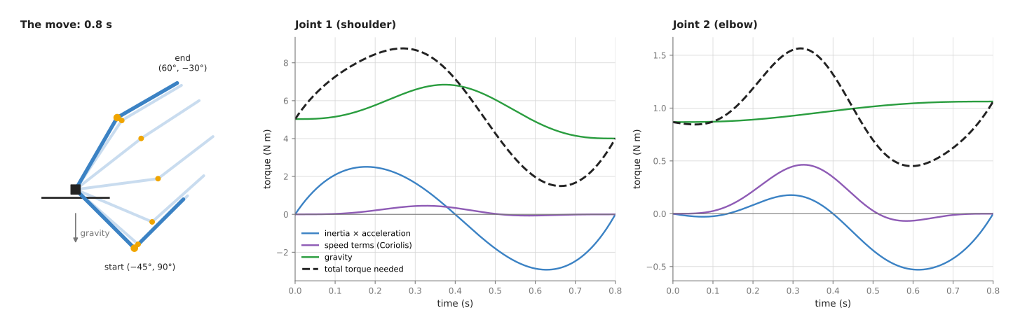
The left panel shows the move itself, while the two charts show, for each joint, the three parts as coloured lines and their sum as a dashed black line.
Read the shoulder chart first. Gravity is the largest part the whole time, at between 4.0 and 6.8 N m, while the inertia part is between −2.9 and +2.5 N m. That inertia part is positive while the arm speeds up and negative while it slows down. The speed part is small here, at most 0.45 N m, so the total the shoulder needs goes from 1.5 up to 8.8 N m.
The elbow chart looks different. Its gravity part is small and steady, at about 0.9 to 1.1 N m. But its speed part reaches 0.46 N m, which is almost as large as the inertia part and half of gravity. So on the lighter, outer joints of an arm, the speed part cannot be ignored on a fast move.
A worked example: one instant by hand#
Since the three parts are easier to trust once you have seen them worked out, here is the torque at one instant, done by hand. The arm is at q1 = 30° and q2 = 45°, while the shoulder is turning at 1 rad/s and the elbow at 2 rad/s. So we want the shoulder to speed up at 3 rad/s² and the elbow to slow down at 2 rad/s². The numbers below all come from the script.
First the mass matrix at this pose:
M = | 0.2239  0.0473 |
    | 0.0473  0.0208 |       (kg m²)
The inertia part is M times the acceleration:
- shoulder: 0.2239 × 3 + 0.0473 × (−2) = 0.5769 N m
- elbow: 0.0473 × 3 + 0.0208 × (−2) = 0.1004 N m
The speed part uses one number, h = m2 × L1 × (distance to link 2's centre of mass) × sin(q2) = 1.0 × 0.30 × 0.125 × sin 45° = 0.0265 kg m²:
- shoulder: −h × (2 × 1 × 2 + 2²) = −0.0265 × 8 = −0.2121 N m
- elbow: h × 1² = 0.0265 N m
The gravity part:
- elbow: 1.0 kg × 0.125 m × 9.81 × cos(30° + 45°) = 0.3174 N m
- shoulder: (2.0 × 0.15 + 1.0 × 0.30) × 9.81 × cos 30° + 0.3174 = 5.4148 N m
The totals are 0.5769 − 0.2121 + 5.4148 = 5.7796 N m at the shoulder and 0.1004 + 0.0265 + 0.3174 = 0.4443 N m at the elbow. This means more than nine tenths of the shoulder's torque is holding the arm up, even in the middle of a move.
The script also computes the same torques a second way, with the recursive Newton–Euler algorithm. It works outwards from the base, link by link, to find each link's acceleration. Then it works back inwards, adding up the force each joint must pass on to the links beyond it. That is the method most libraries use, because it works for any number of joints. It gives 5.7796 and 0.4443 too, and along the whole move the two methods never differ by more than 0.000000000000004 N m.
Inverse and forward dynamics#
That same equation can be used in two directions, and each direction has its own name.
Inverse dynamics goes from motion to torques. You give it the angles, the speeds and the accelerations you want, and it gives back the torque each joint needs. The worked example above is inverse dynamics, and a controller uses it to decide what to send to the motors.
Forward dynamics goes the other way, from torques to motion. You give it the angles, the speeds and the torques, and it gives back the accelerations that will result. To find them, it solves the equation for the acceleration:
acceleration = M(q)⁻¹ × (torque − c(q, speed) − g(q))
The ⁻¹ means "undo the matrix", which a program does by solving two equations in
two unknowns. So when it is fed the 5.7796 and 0.4443 N m from the worked example,
forward dynamics gives back exactly 3 and −2 rad/s².
Forward dynamics is also what a simulator does, because it starts from a pose, works out the accelerations, moves the arm on by a tiny step of time, and repeats. The left panel of the next picture shows forward dynamics with zero torque, where the arm starts still at (30°, 45°) and the motors are switched off.
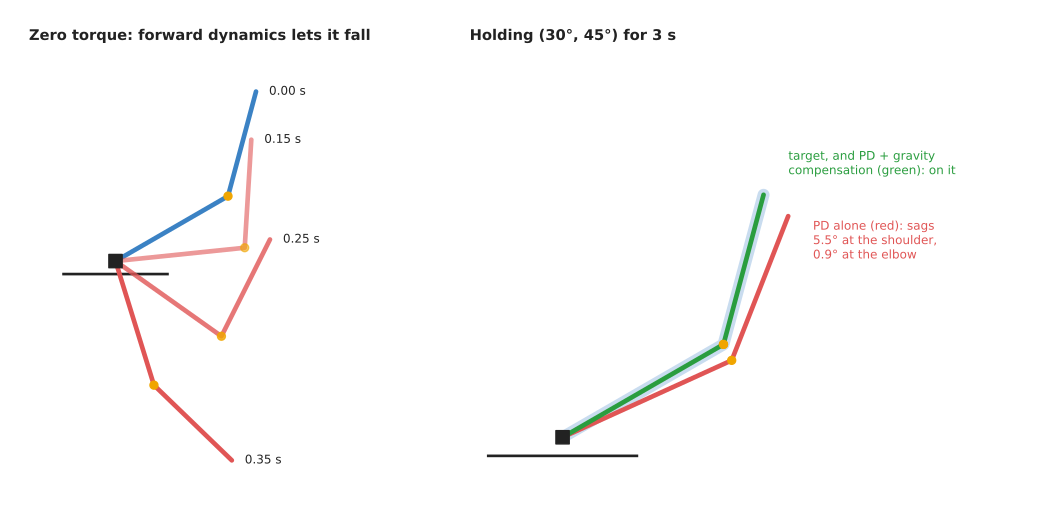
The arm does not simply drop as a stiff stick would. After 0.15 s the shoulder has fallen to 5.9°, but the elbow has bent up from 45° to 80.6°. Then after 0.25 s the shoulder is at −35.4° and the elbow at 98.7°. This happens because the falling upper link flings the lower link round, and that folding comes from the off-diagonal numbers in the mass matrix and from the speed part. So a controller that treats each joint on its own knows nothing about it.
Gravity compensation: holding still with no error#
The simplest use of that equation is the one where nothing moves at all. When the arm is still, the speed and the acceleration are both zero, so the equation shrinks to a single part:
torque needed to hold still = g(q)
Adding g(q) to the controller's output is called gravity compensation, and the PID page describes it in one paragraph. The right panel of the picture above shows what it does.
A proportional-derivative (PD) controller, meaning a PID with no integral term, holds the arm at (30°, 45°) for 3 seconds, and the pale blue arm is the target. Without gravity compensation the red arm sags 5.5° at the shoulder and 0.9° at the elbow. This is because a PD controller only pushes when there is an error, so it must keep an error to hold the arm up, just as the P controller did on the PID page. With gravity compensation, however, the green arm sits exactly on the target with no error at all. The torque it sends is 5.4148 N m at the shoulder and 0.3174 N m at the elbow, which is g(q) at that pose. So the feedback part of the controller has nothing left to do.
An integral term could also remove the sag, by slowly finding the same 5.4 N m. But it takes time to find it, and it must find it again every time the pose changes, because g(q) changes with the pose. Gravity compensation, in contrast, gives the right answer at every pose at once.
Gravity compensation is also how a hand-guided arm works. If the controller sends g(q) and nothing else, the arm floats, so a person can push it anywhere and it stays where it is left. This is the "free drive" or "teach" mode of many arms.
Feed-forward plus PID, and computed-torque control#
Once the arm moves, gravity alone is not enough, so there are two common ways to use the whole model instead.
The first is feed-forward plus PID. The controller works out the torque that the planned motion needs, using inverse dynamics, and adds it to the output of an ordinary PID loop on each joint. This means the model supplies nearly all of the torque and the PID supplies only the rest.
The second is computed-torque control. Here the controller first works out, from the errors, the acceleration it wants each joint to have. That is the planned acceleration, plus a spring-like pull towards the planned angle, plus a damper-like pull towards the planned speed. Then it uses inverse dynamics, at the arm's measured pose and speed, to turn that acceleration into torques. Because the mass matrix is inside the loop, the same two gains give the same behaviour at every pose, and in this example both joints are tuned to respond at 20 radians per second.
The picture below runs the same 0.8-second move four times, each time with a different controller, and shows the error of each joint.
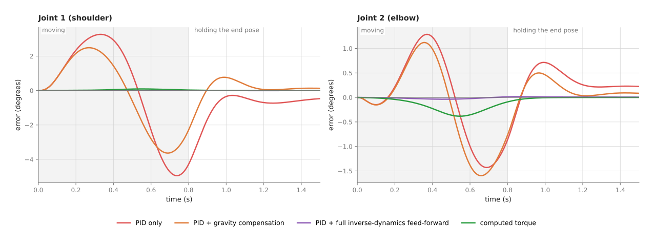
The grey area is the move itself, while the white area after it is 0.7 seconds of holding the end pose. The PID-only run starts with its integral already holding the arm up at the start pose, as it would after standing there for a while.
The table below collects those four runs so that they can be compared directly. Read each row as one controller. The columns give the largest error of each joint during the move, and then the error of each joint at the end of the hold.
| Controller | Largest shoulder error | Largest elbow error | Shoulder error at the end | Elbow error at the end |
|---|---|---|---|---|
| PID only | 4.95° | 1.43° | 0.47° | 0.22° |
| PID + gravity compensation | 3.63° | 1.60° | 0.13° | 0.09° |
| PID + full inverse-dynamics feed-forward | 0.009° | 0.036° | 0.003° | 0.006° |
| Computed torque | 0.092° | 0.38° | less than 0.0001° | less than 0.0001° |
Gravity compensation alone helps the shoulder and the hold, but it does not help much while the arm is moving, and at the elbow it is even slightly worse. This happens because most of the moving error comes from the inertia and speed parts, which gravity compensation leaves out. So the two controllers that use the whole model do much better: at the shoulder they cut the largest error by 50 to 500 times, while at the elbow feed-forward cuts it by 40 times and computed torque by about 4 times. The error they do leave comes from the friction value that is 20 per cent too low. But the computed-torque run shows it more than the feed-forward run, because it has no integral term to slowly push it away.
A payload changes the numbers#
All the numbers above are for an empty gripper. But a payload, meaning whatever the gripper is holding, adds mass at the very end of the arm, where it has the most leverage. A 0.5 kg payload at the tip of this arm is only one sixth of the arm's own 3 kg. Yet it raises the gravity torque at (30°, 45°) from 5.41 to 7.01 N m at the shoulder, and from 0.32 to 0.63 N m at the elbow, so the elbow's number doubles. On the 0.8-second move, the largest torque the shoulder needs rises from 8.8 to 12.1 N m.
So if the controller's model does not know about the payload, it sends the wrong torque. The left panel below runs computed-torque control on the move with the 0.5 kg payload in the gripper.
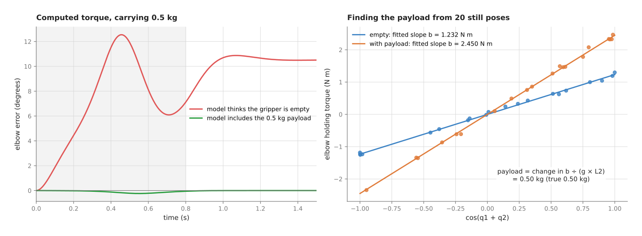
When the model thinks the gripper is empty, the elbow falls behind by up to 12.5° during the move, it is still 10.5° low at the end of the hold, and the shoulder ends 1.1° off. But when the model is told about the payload, the largest elbow error is 0.24° and the end error is zero.
This is why arm makers ask you to enter the payload's mass and where its centre of mass sits, and why a gripper that picks up objects of different weights needs the controller to be told each time, or else a feedback loop with an integral term to absorb the difference.
Finding the arm's masses#
Everything above needs the masses, the centres of mass and the inertias of the links. The arm maker's description gives values for them, but they are often rounded, and they do not include your gripper, your cables or your payload. So measuring them on the real arm has a name of its own: identification.
The key fact that makes identification easy is that the torque is a sum of known terms, each multiplied by an unknown number made from the masses. For the gravity part of this arm, it looks like this:
g1 = a × cos(q1) + b × cos(q1 + q2)
g2 =               b × cos(q1 + q2)
Here a = (m1 × lc1 + m2 × L1) × 9.81 and b = m2 × lc2 × 9.81, where lc1 and lc2 are the distances from each joint to its link's centre of mass. The cosines can be worked out from the measured angles, so only a and b are unknown. That makes it a straight-line fit, which is the same problem the least-squares fitting page solves.
The right panel of the picture shows that fit done. The arm stops at 20 random poses and records the torque each joint uses to hold still, with sensor noise of 0.05 N m added. So each dot in the panel is one pose. Plotted against cos(q1 + q2), the elbow's torques lie on a straight line through zero whose slope is b. The fit gives b = 1.232 N m with the gripper empty (the true value is 1.226) and b = 2.450 N m with the payload (true 2.453). So the payload's mass is the change in b divided by 9.81 × 0.25 m, which gives 0.50 kg, the true value.
The inertias need more work, because they only show up when the arm accelerates. The usual method runs the arm along a special path that shakes every joint at several speeds, called an exciting trajectory. Then it records the angles and motor currents, and fits all the unknowns at once with least squares. The system identification page explains this in general. Friction is fitted at the same time, with its own unknown numbers.
The steps as pseudocode#
Once all those pieces are in place, the whole method fits in a page of pseudocode. The code below uses plain names, so it works in any language, and the first part is inverse dynamics for the two-joint arm. A general library does the same job with the recursive Newton–Euler algorithm, for any number of joints.
inverse_dynamics(q, speed, accel):
    M      = mass_matrix(q)                 # 2 × 2 table, depends on q2
    h      = m2 * L1 * lc2 * sin(q2)
    c      = [ -h * (2 * speed1 * speed2 + speed2^2),
                h * speed1^2 ]
    g2     = m2 * lc2 * 9.81 * cos(q1 + q2)
    g      = [ (m1 * lc1 + m2 * L1) * 9.81 * cos(q1) + g2,  g2 ]
    return M * accel + c + g
The second part is forward dynamics, as a simulator uses it: one small step of time.
simulate_one_step(q, speed, torque, step):
    accel = solve( mass_matrix(q), torque - c(q, speed) - g(q) )
    speed = speed + accel * step
    q     = q + speed * step
    return q, speed
The third part is the two controllers, run once per tick.
every tick:
    (q_plan, speed_plan, accel_plan) = trajectory at this time
    (q, speed) = read_encoders()
    error      = q_plan - q
    error_rate = speed_plan - speed

    # feed-forward plus PID
    torque = inverse_dynamics(q_plan, speed_plan, accel_plan) + pid(error)

    # or computed torque
    wanted = accel_plan + Kp * error + Kd * error_rate
    torque = inverse_dynamics(q, speed, wanted)

    send torque to the motors
Gravity compensation alone is the last line of inverse_dynamics with only g
returned, added to a PD or PID output.
4. Where it is used on a robot arm#
Because a dynamics model answers both "what torque?" and "what motion?", it turns up in many places on and around an arm, and the list below gives the main ones.
Inside the drives of torque-controlled arms. Collaborative arms such as the Franka
arms and the KUKA LBR iiwa run gravity compensation and dynamics feed-forward inside
their controllers. So libfranka's franka::Model class gives a program the arm's mass
matrix, its Coriolis torques and its gravity torques at the current pose, which a
user's own torque controller can then use.
Hand guiding and teaching. The "free drive" button on many arms switches to pure gravity compensation. The arm holds itself up, and a person moves it by hand to teach it poses.
Impedance control. An impedance controller makes the arm act like a soft spring, but it only works if gravity is compensated, because otherwise the soft arm sags. The impedance and force control page says that if the gravity model is wrong the arm drifts as soon as it is made soft; this page is where that model comes from.
Collision detection. A collision detector compares the torque each joint is actually using with the torque that inverse dynamics says it should need. So a large gap means something the model does not know about is pushing on the arm, such as a person. Book 7's collision and failure detection page calls this the "expected torque". The better the model, the lower the alarm line can be set. The safety monitoring page covers the checks that act on such alarms.
Simulators. Gazebo, MuJoCo, Drake and Isaac Sim all run forward dynamics, a thousand or more times per simulated second, to move a simulated arm. So a policy trained in simulation, as described in Book 6, only works on the real arm if the simulator's masses are close to the real ones.
Checking a trajectory before running it. Inverse dynamics along a planned move gives the torque each motor will need. So if that is above a motor's limit, the move must be slowed down before it is sent. That is why time-parameterisation tools such as TOPP-RA, named on the trajectory generation page, can take torque limits.
Payload checks. After a grasp, the arm can hold still for a moment and compare its joint torques with the gravity model. The difference then tells it the mass of what it picked up, as in the identification example, so a result of zero means the grasp missed.
5. Where it is useful, and where it is not#
The uses above are not all equally worthwhile, because a dynamics model helps most on fast moves, heavy arms, soft (impedance) control and collision detection. It helps least on slow moves of a stiff, geared, position-controlled arm, where the drive's own PID loops already keep the error small.
The table below lists the common failures. Read each row as one situation, giving the sign you would see and what people use instead or add to fix it.
| Situation | The sign you would see | What people use instead or add |
|---|---|---|
| The payload in the model is wrong or missing | the arm sags or lags after a grasp; false collision alarms while carrying a load | set the payload in the controller after each grasp; estimate it from the holding torques; keep an integral term |
| Friction in the gearboxes is large, as in most geared arms | the model's torque is right in theory but the arm still lags, worst when it starts or reverses | identify a friction model with the masses; a learned arm model for the part physics leaves out |
| Cables, hoses and springs pull on the arm | a steady error that changes with pose but not with load | identify the pull as an extra term; a learned correction |
| The link masses in the description are rounded or wrong | gravity compensation leaves a small sag that changes with pose | identification from still poses and an exciting trajectory |
| The links or gearboxes bend | the arm rings after fast moves even with an accurate model | lower speeds and smoother trajectories; a flexible-joint model |
| The arm touches something | the model's torque no longer matches, because the contact force is missing from it | impedance and force control, and a force sensor |
| The arm only accepts position commands | there is no place to send a computed torque | use the dynamics only for checks and collision detection; leave control to the drive |
The last row of that table matters most in practice. Many industrial arms, and most low-cost ones, only accept joint positions, because their drives do their own control inside. So on such an arm you can still use dynamics to check torques and detect collisions, but you cannot send the controller's torque yourself.
6. Libraries that provide it#
Since the equations grow quickly with the number of joints, you almost never write dynamics by hand for a real arm. Instead you give a library the arm's description, usually a Unified Robot Description Format (URDF) file, which lists each link's mass, centre of mass and inertia, and the library does the rest. The table below lists the well-known ones. Read each row as one library, giving the languages it is used from, the functions to call, and a note on what it is for.
| Library | Languages | Functions or classes | Note |
|---|---|---|---|
| Pinocchio | C++, Python | rnea (inverse dynamics), aba (forward dynamics), crba (mass matrix), computeGeneralizedGravity, nonLinearEffects, computeJointTorqueRegressor | fast and widely used; the regressor function gives the table of known terms used for identification |
| Drake | C++, Python | MultibodyPlant.CalcInverseDynamics, CalcMassMatrix, CalcBiasTerm, CalcGravityGeneralizedForces; the InverseDynamicsController system | a full simulator and planning toolbox; note that CalcGravityGeneralizedForces returns the force gravity applies, so the holding torque is its negative |
| KDL (Orocos Kinematics and Dynamics Library) | C++, Python | ChainIdSolver_RNE (inverse dynamics), ChainDynParam with JntToMass, JntToCoriolis, JntToGravity | older but still common in ROS code |
| MuJoCo | C, Python | mj_inverse, mj_step; the qfrc_bias field holds gravity plus speed terms | a simulator, often used for learning; its inverse dynamics is used for checks |
| RBDL (Rigid Body Dynamics Library) | C++, Python | InverseDynamics, ForwardDynamics, NonlinearEffects | a small library with the same algorithms |
| libfranka | C++ | franka::Model with mass, coriolis, gravity | the Franka arm's own model, identified by the maker |
For identification there are dedicated tools built on these as well. But the core of
it is a least-squares fit, which NumPy's numpy.linalg.lstsq does in one call, as the
diagram script shows.
7. Why a dynamics model, and what it costs#
To put all of the above together, a dynamics model is the set of equations that link the torques at the joints to the arm's motion. This means it gives a controller most of the torque each joint needs before any error appears, holds the arm still against gravity with no error at all, and lets a simulator predict what the real arm will do.
The obvious alternative is to use no model and let the feedback loop do all the work, with higher gains or a stronger integral term. That is what most position-controlled arms do, and on slow moves it works. But feedback only corrects an error after it has appeared, so the error grows with speed. In the example on this page, PID alone left a 4.95° error at the shoulder on a 0.8-second move. But adding the model cut that to 0.009°, with the same PID gains. Higher gains would shrink the error too, but they make the arm stiff and noisy, and they push harder on anything it touches, which is the wrong direction for an arm that works near people.
The second alternative is a learned model of the arm. Section 8 says why the usual practice is to use both.
The costs are these. You need the masses, centres of mass and inertias of every link, and the maker's values may be rough, while you must also tell the controller about every payload. The model leaves out friction, cables and bending unless you add them. The equations are hard to check by hand beyond two or three joints, so you depend on a library and on a correct URDF file. And the full benefit needs an arm that accepts torque commands, which many arms do not.
8. The learned alternative#
Book 7's learned arm models are the learned version of this page. Most keep this physics model and add a small network that learns only what is left over: the gearbox friction, cable pull and wear that the equations leave out. A learned correction wins when those effects do not fit a simple number, such as friction that changes with speed and temperature. It also trains on the arm's own recordings, which are cheap and safe to collect. But the physics model still wins as the base, because it needs only a handful of numbers per link and gives sensible answers everywhere. A learned model, in contrast, needs hours of varied data and can give strange answers for moves it has not seen. That is why the usual practice is to keep the physics model and let a learned model correct it. Book 7's learned dynamics models do a wider job: they predict how the whole scene moves when the arm acts, not just the arm.
9. Where to read next#
- PID control is the feedback loop that runs on top of the model on this page and cleans up what the model gets wrong.
- Trajectory generation makes the planned angles, speeds and accelerations that inverse dynamics turns into torques.
- The next page, safety monitoring, covers the software checks that watch the arm's limits, including the torque limits this page computes.
- Impedance and force control uses gravity compensation to make the arm soft on contact.
- Least-squares fitting and system identification explain the fitting used to find the arm's masses.
- Book 3's controlling the move shows where position, stiffness and torque control sit in ROS 2.
10. Using it in Python#
Section 3 split a joint torque into its three parts, worked one instant out by hand, and showed how the same numbers are used as feed-forward next to a PID loop. Section 6 then explained that you give a library the arm's description instead of writing those equations. This section shows the four calls that do it, so that after reading it you can compute a holding torque, a full inverse-dynamics torque and a mass matrix from a Unified Robot Description Format (URDF) file.
The example uses Pinocchio, because it is the fastest of the libraries in section 6 that has a real Python interface, and because it also provides the regressor used for identification.
import numpy as np, pinocchio as pin

model = pin.buildModelFromUrdf("arm.urdf")   # masses, centres of mass and inertias
data = model.createData()                    # scratch space the algorithms reuse

q = np.array([0.4, -0.9])       # joint angles, radians
v = np.zeros(model.nv)          # joint speeds, radians per second
a = np.array([1.0, 0.0])        # the accelerations the trajectory asks for

tau = pin.rnea(model, data, q, v, a)               # inverse dynamics: torque to apply
g = pin.computeGeneralizedGravity(model, data, q)  # only the part that holds it up
M = pin.crba(model, data, q)                       # the mass matrix
a_result = pin.aba(model, data, q, v, tau)         # forward dynamics, for a simulator
Those four lines are the whole of section 3 in code. pin.rnea returns all three parts
of the torque added together, which is what you send as feed-forward.
computeGeneralizedGravity returns the gravity part alone, which is what gravity
compensation needs. crba returns the mass matrix, which is what computed-torque
control multiplies the PID output by. aba goes the other way, from torques to
accelerations, which is what a simulator needs.
What the library does for you is the algebra and the speed. The equations grow quickly
with the number of joints, but the recursive algorithms behind rnea and aba walk the
chain of links once, so their work grows only in proportion to the number of joints.
That is why they are fast enough to run inside a loop at a thousand ticks a second,
and you never see a term of the equation at all.
What you still write is the arm description and everything around the call. If the
maker publishes a URDF you use it, and if it does not you write it yourself, link by
link. The loop is yours, reading q and v from the arm and sending tau to it. And
the feed-forward torque on its own is not a controller: you still add the PID output
from the PID page, because the model is
never exact.
What you have to decide or measure is the contents of that URDF, and it is the part
that decides whether the feed-forward helps or hurts. Each link needs a mass, a centre
of mass and an inertia, and section 3 shows how a least-squares fit finds them from
real motion when the maker's numbers are missing. A held object is not in the file, so
either you add it as a link at the tool frame or the model will under-shoot by exactly
its weight, as section 3's payload example shows. Gravity itself is a choice as well:
model.gravity.linear defaults to [0, 0, -9.81], which assumes the arm's base frame
is upright, so an arm bolted to a wall or a ceiling needs that vector changed or every
gravity torque will be wrong.