This page explains optimisation solvers, which are general programs that find the best choice among a very large number of choices while obeying rules you give them, and it answers five questions. What do you have to tell a solver, and what are linear, integer and constraint programming, and how do they differ? How does a solver find the best answer without trying every possibility? And where does a robot arm need one, and when is a simple loop, or a greedy rule, the better tool?
It is written for a reader who has read greedy algorithms and set cover, because that page showed a quick rule that is usually close to the best answer. This page is instead about getting the best answer itself, and about what that costs. No mathematics beyond adding and multiplying is needed, since the page explains each term where it first appears.
On a robot arm, solvers answer questions about tasks rather than about motion. Which part goes into which pocket of a tray, and in what order should the arm pick five objects when one of them blocks another? How many of each item fit in a box before it is too heavy? These are the questions in the worked examples below.
Contents#
- The idea in one sentence
- What you tell a solver, and the three main kinds
- How it works, with three worked examples · Assignment: which part goes in which pocket · Ordering: which object to pick first, with a rule · Packing: why rounding a fractional answer fails · Branch and bound: how an integer solver avoids trying everything · When trying everything stops working
- Where solvers are used on a robot arm
- Where a solver is useful, and where it is not
- Libraries that provide it
- Why a solver, and what it costs
- The learned alternative
- Where to read next
- Using it in Python
1. The idea in one sentence#
Since greedy gives up the best answer for speed, here is the tool that does not. An optimisation solver is a ready-made program that takes a description of your choices, your rules and your score, and returns the choice that obeys every rule and has the best score.
Here is an everyday example of such a program, a school that has to make a timetable. The choices are which teacher teaches which class in which room at which hour, while the rules are that no teacher is in two rooms at once, no room holds two classes at once, and every class gets its hours of each subject. The score might be the number of free gaps in the teachers' days, which the school wants as small as possible. But nobody writes a special program for this school. Instead they write the choices, rules and score in the form a timetable solver accepts, and then the solver finds the timetable.
That same split is what makes a solver useful on a robot, because you describe the task and the solver does the searching. So when the task changes, for example when a new rule says that one object must be picked before another, you add one line to the description rather than a new search algorithm.
2. What you tell a solver, and the three main kinds#
Because you describe the problem rather than the search, every problem you give a solver has the same three parts. The words below are the standard ones, and every solver's documentation uses them.
- The decision variables are the choices the solver makes. For example, "does part 1 go into pocket 3?", with the answer 1 for yes and 0 for no.
- The constraints are the rules every answer must obey. For example, "each pocket holds exactly one part".
- The objective is the score. For example, "the total distance the arm travels", which the solver makes as small as possible.
Writing these three parts down is called modelling, and the result is called the model. So the model is the part you write, while the solver is the part you install.
There are three main kinds of solver, and they differ in what the variables and rules are allowed to look like. The table below compares them, so read each row as one kind, giving what its variables can be, what its rules can be, and the robot questions it suits.
| Kind | Variables | Rules and score | Suits |
|---|---|---|---|
| Linear programming (LP) | Any number, fractions allowed | Sums of variables times fixed numbers, compared with ≤, = or ≥ | Blending and sharing amounts: how much time each arm spends on each job |
| Mixed-integer linear programming (MILP, often shortened to MIP) | Some must be whole numbers, often 0 or 1 | The same sums as LP | Yes-or-no choices: which part to which pocket, which views to use, how many boxes |
| Constraint programming (CP) | Whole numbers from a list of allowed values | Almost any rule: "all different", "A before B", "if this then that" | Orders, schedules and puzzles with many logical rules |
The word "programming" in these names is old, and it means "planning" rather than writing code. Linear programming was named in the 1940s, when a "programme" was a military plan.
A fourth kind, nonlinear optimisation, allows curved rules and scores, such as the distance between two joint positions, so it is what trajectory optimisation and numerical inverse kinematics use. Those two have their own pages: trajectory optimisation and numerical inverse kinematics. This page stays with the first three, which are the ones used for task decisions.
3. How it works, with three worked examples#
Because the three parts are easier to see on a real task, each example below is small enough that the diagram script solves it exactly by trying every possibility. That gives a true best answer to compare against, and every number on this page comes from that script.
Assignment: which part goes in which pocket#
Four parts, P1 to P4, lie on a table, and a kit tray at the front edge has four pockets, T1 to T4. The arm must put one part in each pocket, and the score is the total straight-line distance from each part to its pocket, in millimetres. This kind of problem is called an assignment problem.
The table below gives the distance from each part to each pocket. Read each row as one part, and each column as one pocket.
| T1 | T2 | T3 | T4 | |
|---|---|---|---|---|
| P1 | 193.1 | 247.6 | 324.5 | 411.5 |
| P2 | 130.0 | 130.0 | 192.1 | 277.3 |
| P3 | 180.3 | 111.8 | 111.8 | 180.3 |
| P4 | 277.3 | 192.1 | 130.0 | 130.0 |
As a model, this problem has 16 yes-or-no variables and 8 rules:
decisions:  x[i][j] = 1 if part i goes to pocket j, otherwise 0
rules:      for each part i:    x[i][1] + x[i][2] + x[i][3] + x[i][4] = 1
            for each pocket j:  x[1][j] + x[2][j] + x[3][j] + x[4][j] = 1
score:      minimise the sum over all i and j of distance[i][j] × x[i][j]
There are 4 × 3 × 2 × 1 = 24 ways to assign four parts to four pockets, and trying all 24 gives the best one: P1 to T1, P2 to T2, P3 to T3 and P4 to T4, for a total of 564.9 mm. The worst of the 24 is 992.7 mm.
But the greedy rule, "take the closest remaining part and pocket first", does much worse. Its first choice is P3 to T2, at 111.8 mm, which is the smallest number in the table. Then it takes P2 to T1 and P4 to T3, both at 130.0 mm, and that leaves P1 with only T4, the most distant pocket, at 411.5 mm. So the total is 783.3 mm, which is 39 per cent more than the best. The picture below shows both answers.
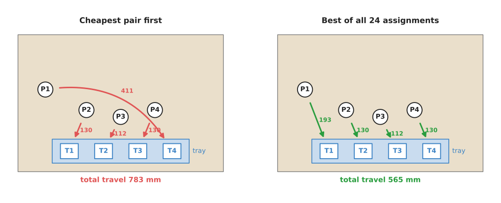
The number on each arrow is that part's distance to its pocket in millimetres, while the curved arrow on the left is the 411.5 mm move that greedy is left with at the end.
The assignment problem does have a special property, however, because it has its own exact method, the Hungarian algorithm, which is fast even for hundreds of parts. Assignment and matching explains it. So in practice you would not call a general solver for this exact problem. Instead you would call one as soon as a rule is added that the Hungarian algorithm cannot express, such as "P2 and P3 must not go into neighbouring pockets, because the gripper cannot fit between them".
Ordering: which object to pick first, with a rule#
The assignment above had no rules beyond one part per pocket, so the next example adds one. Five objects, A to E, stand on the table, and the arm starts at the front left corner, picks all five, and ends at a bin at the front right corner. The score is again the total straight-line travel, but now there is one rule: object C stands in front of object B and blocks the gripper's approach, so C must be picked before B.
There are 5 × 4 × 3 × 2 × 1 = 120 orders, and exactly half of them, 60, pick C before B. The picture below shows three of those orders.
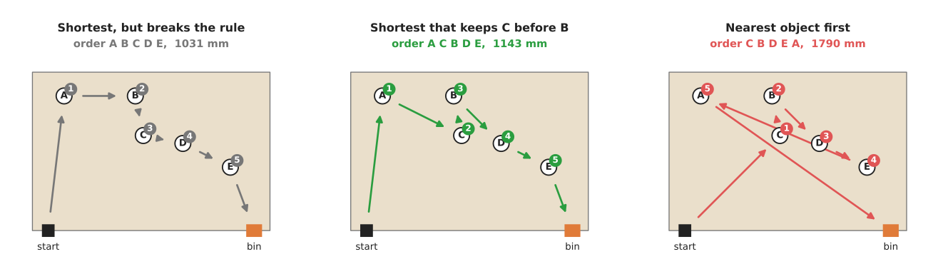
The small numbered circles give the order of the picks, while the black square is where the arm starts and the orange square is the bin.
The table below lists the results, and each row is one way of choosing the order.
| How the order was chosen | Order | Travel |
|---|---|---|
| Shortest of all 120, ignoring the rule | A B C D E | 1031.3 mm |
| Shortest of the 60 that pick C before B | A C B D E | 1142.7 mm |
| Nearest object first, among those not blocked | C B D E A | 1790.4 mm |
| Longest of the 60 that pick C before B | C E A D B | 1976.7 mm |
The shortest order breaks the rule, so it cannot be used, and the best allowed order costs 111.4 mm more. Meanwhile the nearest-first greedy rule is 57 per cent longer than the best allowed order. Its first pick, C, is 339 mm from the start and A is 342 mm, so C wins by only 3 mm. Then greedy works its way to the right, and it has to come all the way back for A at the end.
This is the point of a solver. The rule "C before B" is one line in a model, whereas in a hand-written search it is a special case you have to remember to check. And a greedy rule can respect it only by refusing to pick B early, which does nothing to make the rest of its route good.
Book 3's ordering and rearrangement shows how to find rules like "C before B" from the scene, using a blocking graph. So the solver's job starts where that page's job ends, because once the rules are known it finds the shortest order that obeys them.
Packing: why rounding a fractional answer fails#
Both examples above chose between whole things, and the third example shows why whole-number problems are harder than fractional ones.
An arm fills a shipping box that holds at most 6 items and at most 45 kg. A small item weighs 5 kg and is worth 5, while a large item weighs 9 kg and is worth 8. So how many of each should go in, to make the box worth the most?
decisions:  s = number of small items, l = number of large items (whole numbers)
rules:      s + l ≤ 6
            5 × s + 9 × l ≤ 45
score:      maximise 5 × s + 8 × l
The picture below draws that problem, where each axis counts one kind of item. Each rule is a straight line, and the allowed answers lie below both lines.
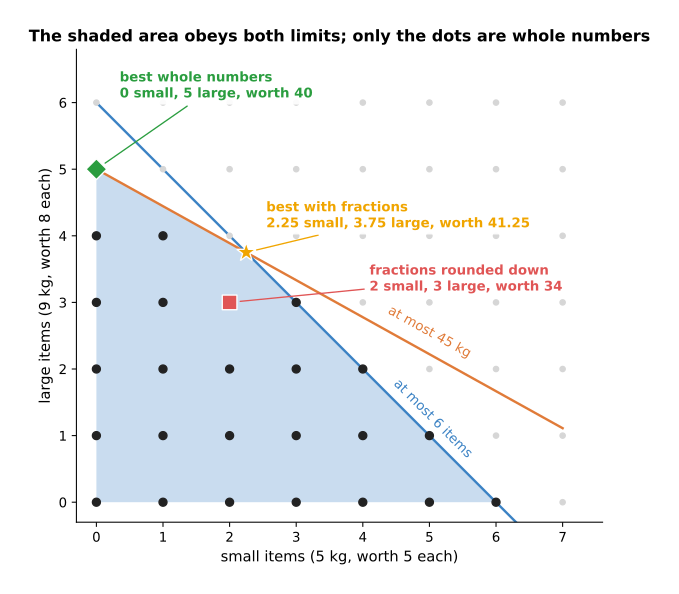
The shaded area is what obeys both rules if fractions of an item were allowed, while the black dots are the 25 whole-number answers that obey both rules.
If fractions were allowed, the problem would be a linear program, and a linear program has a useful property: its best answer can always be found at a corner of the shaded area, where two rule lines meet. So a linear programming solver only has to look at the corners. Here the best corner is where both rules are exactly met, at 2.25 small and 3.75 large items, worth 41.25.
The obvious next step is to round that down to whole numbers, giving 2 small and 3 large. That obeys both rules, but it is worth only 34, while the best whole-number answer is 0 small and 5 large, worth 40. So it is not next to the fractional answer at all.
This is why integer problems need more than a linear programming solver and a rounding step, because the best whole-number answer can be far from the best fractional one.
Branch and bound: how an integer solver avoids trying everything#
Since rounding fails, an integer solver uses the fractional answer as a guide rather than as the answer. The standard method for doing that is called branch and bound, and it has four steps.
- Solve the problem with fractions allowed. This is fast, because only corners need checking. Its score is a bound: no whole-number answer can beat it.
- If the answer is already whole numbers, it is a candidate. Keep the best candidate found so far.
- If some variable is a fraction, such as
l = 3.75, split the problem into two smaller problems: one with the extra rulel ≤ 3, one withl ≥ 4. Every whole-number answer is in one of the two. This split is the branch. - Solve each smaller problem the same way. If a problem's fractional score is no better than the best candidate so far, drop it without looking inside. No answer inside it can win.
On the packing example above it runs like this, and every number comes from a real run.
- The whole problem, with fractions: 41.25, at 2.25 small and 3.75 large. Split on the large count.
- With
l ≤ 3: the fractional best is 39, at 3 small and 3 large. These are whole numbers, so this is the first candidate, worth 39. - With
l ≥ 4: the fractional best is 41, at 1.8 small and 4 large. That could still beat 39, so split on the small count. - With
l ≥ 4ands ≥ 2: no answer obeys the weight rule. Drop it. - With
l ≥ 4ands ≤ 1: the fractional best is 40.56, at 1 small and 4.44 large. It could still beat 39, so split on the large count again. - With
s ≤ 1andlexactly 4: the best is 37. That cannot beat 39. Drop it. - With
s ≤ 1andl ≥ 5: the best is 40, at 0 small and 5 large, in whole numbers. That beats 39 and becomes the answer.
So the solver solved seven small fractional problems and proved that 40 is the best. On a problem this size that saves nothing over checking all 25 dots. But on a problem with hundreds of variables, the dropping in step 4 is what makes the difference between seconds and years. Real solvers add many refinements to this idea, and they all rest on it.
Here are the same steps written as pseudocode:
branch_and_bound(problem):
    best = none
    to_do = [problem]
    while to_do is not empty:
        p = take one problem from to_do
        fractional = solve p with fractions allowed
        if p has no answer:                           continue
        if best is not none and fractional.score is no better than best.score:
            continue                                  # nothing in here can win
        if every whole-number variable in fractional is a whole number:
            best = fractional                         # a new best candidate
            continue
        v = a variable with a fractional value f in fractional
        add (p with rule v ≤ floor(f)) to to_do
        add (p with rule v ≥ floor(f) + 1) to to_do
    return best
A constraint programming solver searches differently. It keeps, for every variable, the list of values that are still possible, and each rule removes the values that can no longer work. For example, in the ordering example above, "C before B" means C can never be in the last position and B can never be in the first. Removing impossible values this way is called propagation. Then, when the rules can remove nothing more, the solver tries one value for one variable, propagates again, and backs up if it reaches a dead end. Modern solvers such as OR-Tools' CP-SAT combine this with the integer methods above.
When trying everything stops working#
Each example above was solved by trying every possibility, which is the right method for small problems, because it is short, it is exact, and it cannot have a bug in its search. But the trouble is how quickly the number of possibilities grows.
With n places to visit, there are n × (n − 1) × ... × 2 × 1 orders, written n!
and read "n factorial". A plain Python loop on the machine this page was written on
checked about 630,000 orders a second, so with ten places it took 5.76 seconds to
check all 3,628,800 orders. The chart below shows what that rate means for other
sizes.
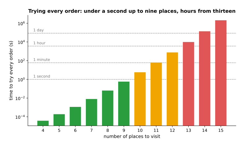
Each bar is the time to check every order at 630,000 orders a second, drawn on a logarithmic scale where each step up is ten times longer. Green is under a second, orange is under an hour, and red is longer than that.
The table below gives the same numbers for a few sizes, so read each row as the number of places, the number of orders, and the time to try them all.
| Places | Orders | Time to try every order |
|---|---|---|
| 5 | 120 | under a millisecond |
| 8 | 40,320 | 0.06 s |
| 10 | 3,628,800 | 5.8 s |
| 12 | 479,001,600 | 760 s, about 13 minutes |
| 13 | 6,227,020,800 | 9,884 s, about 2.7 hours |
| 15 | 1,307,674,368,000 | 2,075,674 s, about 24 days |
A faster language would move every bar down by a factor of perhaps a hundred, but it would not change the shape, because each extra place multiplies the work by the number of places. That is where a solver earns its place, since it uses bounds and propagation to skip most of the possibilities. So it can solve problems far past the point where trying everything is hopeless.
4. Where solvers are used on a robot arm#
Because a solver plans a whole set of choices at once, solvers are used for decisions about a whole task, made before the arm moves or between moves. Here are the common places.
- Filling a kit tray. Which part goes into which pocket, as in the first example. Rules like "heavy parts in the bottom row" or "no two tall parts side by side" make it a job for an integer or constraint solver rather than the Hungarian algorithm.
- Pick order with blocking rules. The order in which to clear a cluttered table, as in the second example. The rules come from Book 3's blocking graph. The solver finds the shortest order that obeys them.
- Sharing work between two arms. Which arm picks which object, and in what order, so that both finish early and never reach into the same space at the same time. The "same space at the same time" rule is a scheduling rule, which constraint programming handles well.
- Palletising and box packing. Which box goes where on a pallet, subject to weight, size and stacking rules, as in the third example but with positions as well as counts.
- Choosing camera views exactly. The set cover problem from greedy algorithms and set cover, written as an integer program: one yes-or-no variable per view, one rule per object ("at least one chosen view sees it"), and the score "number of views chosen". This finds the true smallest set when greedy is not good enough.
- Scheduling tool changes and machine loading. When the arm serves several machines, which job to load next so that no machine waits, and when to change the gripper.
- Allocating a time budget. A linear program can split a fixed cycle time between inspection, picking and placing, when each has a known effect on the score.
Nonlinear solvers, which are a different family, also run inside motion planning, because they smooth a path in trajectory optimisation and find joint angles in numerical inverse kinematics.
5. Where a solver is useful, and where it is not#
The uses above all share one condition, because a solver is useful when there are many choices, when the rules matter, and when the difference between a good answer and the best one is worth real time or money. But it is less useful when the problem is tiny, when the scene changes after every move, or when the model leaves out something important.
The table below lists the common problems. Read each row as one situation, giving the sign you would see and what to do instead.
| Situation | What you would see | What to do instead |
|---|---|---|
| The problem is tiny, such as fewer than about eight objects | The solver takes longer to start than a loop takes to try every order | Try every possibility in a plain loop |
| The scene changes after every pick | The best order is recomputed each time, and only its first step is used | A greedy rule, or a solver with a short time limit |
| The model leaves out a rule, such as a joint limit or a collision | The solver's best answer cannot be carried out on the arm | Add the rule to the model; check each answer with the motion planner before moving |
| Straight-line distance stands in for arm travel time | The "shortest" order is not the fastest on the real arm | Measure move times between places and use those in the model |
| The problem is large and the time budget short | The solver runs until its time limit and returns its best answer so far, without proof | Accept a good answer: set a time limit, and start from a greedy answer |
| Rules contradict each other | The solver reports that no answer exists | Find the smallest set of clashing rules; some solvers can report it |
| The rule is really a preference, such as "try to pick red first" | No answer, or a poor one, because a wish was written as a hard rule | Move the preference into the score with a weight |
One sign is worth knowing in particular. If the solver returns an answer that the arm cannot carry out, the fault is almost never in the solver but in the model. This is because a solver finds the best answer to the problem you wrote, not to the problem you meant.
6. Libraries that provide it#
Optimisation solvers are large, well-tested programs, so almost nobody writes their own. The table below lists the well-known ones, and each row is one library, giving the languages it can be used from, the relevant part, and what it is good for.
| Library | Languages | Function, class or module | Note |
|---|---|---|---|
| Google OR-Tools | C++, Python, Java, C# | ortools.sat.python.cp_model.CpModel and CpSolver (CP-SAT) | The usual first choice for assignment, ordering and scheduling with logical rules |
| Google OR-Tools | C++, Python, Java, C# | ortools.linear_solver.pywraplp.Solver | One interface to several linear and integer solvers |
| Google OR-Tools | C++, Python, Java, C# | pywrapcp.RoutingModel and RoutingIndexManager | Visiting orders, with time windows and capacity rules |
| Google OR-Tools | C++, Python, Java, C# | ortools.graph.python.linear_sum_assignment.SimpleLinearSumAssignment | Fast exact assignment, with no extra rules |
| SciPy | Python | scipy.optimize.linprog, scipy.optimize.milp | Linear and mixed-integer programs, with no extra install beyond SciPy |
| SciPy | Python | scipy.optimize.linear_sum_assignment | Exact assignment, by a method of the same family as the Hungarian algorithm |
| HiGHS | C++, Python (highspy), others | the HiGHS solver | A fast open-source linear and integer solver; SciPy's linprog and milp call it |
| PuLP | Python | pulp.LpProblem, pulp.LpVariable | A simple way to write linear and integer models, then hand them to a solver |
| Pyomo | Python | pyomo.environ.ConcreteModel | A modelling language for larger models, with many solvers behind it |
| MiniZinc | its own modelling language | the MiniZinc tool | A standard language for constraint models, with many solvers behind it |
| CasADi | C++, Python, MATLAB | casadi.Opti, nlpsol | Nonlinear optimisation, used for trajectories rather than task decisions |
Commercial solvers such as Gurobi and CPLEX are also widely used, and they are often faster on very large integer problems, so the modelling tools above can call them.
7. Why a solver, and what it costs#
What it is#
An optimisation solver is a general program that finds the best answer to a problem you describe as choices, rules and a score. The three main kinds are linear programming for fractional amounts, integer programming for yes-or-no and whole-number choices, and constraint programming for orders and logical rules.
What it does for you#
It separates what you want from how to search for it. You write the task, and then a tested program does the search, with bounds that let it skip most of the possibilities. So it gives the best answer, or else tells you how far its answer can be from the best, and new rules are one line each. In the examples above, the solver's answer beat the greedy rule by 39 per cent on the tray and by 57 per cent on the pick order.
Why a solver rather than the obvious alternative#
There are two obvious alternatives, and each wins in its own range. The first is
trying every possibility in a loop, which is exact and has no dependency, so below
about eight to ten items it is the better choice. But the solver wins past that,
because the loop's time grows by a factor of n for every extra item. The second
alternative is a greedy rule, which is fast and simple, and it wins when the scene
changes after every move, because a perfect long plan would then be thrown away
anyway. The solver wins instead when a plan is followed for many steps or many cycles,
or when the rules are what make the task hard. This is because a greedy rule cannot
plan around a rule, and it can only refuse a choice that breaks one.
What it costs you#
It costs a dependency, and time spent learning to model. Writing a good model is a skill, because the same problem can be written in ways that solve in a second or not at all. It also costs predictability of run time, because a hard problem can take much longer than an easy one of the same size, so a robot needs a time limit and a fallback answer. And it costs trust in the model, because the answer is only as good as the rules and the costs you wrote. So straight-line distances, missing collision rules and hard rules that should have been preferences all show up as answers the arm cannot use.
8. The learned alternative#
No model in Book 6 finds the best assignment, order or packing under hard rules. This is because a network gives no proof that its answer obeys every rule, or of how far it is from the best, while a solver gives both. The nearest learned model is a language model as planner, which turns a request in plain words into a sequence of steps. It wins when the task itself changes from day to day and is easier to say than to write as a model, but it can write steps that sound right and are wrong, so its plan needs a checker in ordinary code. A common design uses both: the language model writes the goal and the rules, and a solver finds the order.
9. Where to read next#
- Greedy algorithms and set cover, the page before this one, is the fast approximate alternative.
- Assignment and matching explains the Hungarian algorithm, the special exact method for assignment.
- Trajectory optimisation uses nonlinear optimisation to shape an arm's path.
- Behaviour trees show how the plan a solver produces is carried out step by step, with checks after each step.
- The chapter overview compares all the decision techniques in one table.
- Book 3's ordering and rearrangement explains where ordering rules come from, and why the plan should be recomputed after every move.
10. Using it in Python#
Section 3 wrote the kit-tray assignment as decisions, rules and a score, and section 6 listed the libraries that solve such a model. This section writes that same model in Python twice, so that after reading it you can call a solver on the example from section 3 and you know when the short call is enough and when you need the longer one.
The first version is the short call. SciPy's linear_sum_assignment solves assignment
exactly, and for a bare assignment problem it is all you need.
import numpy as np
from scipy.optimize import linear_sum_assignment

# distance[part][pocket], in millimetres, as in section 3
distance = np.array([[193.1, 247.6, 324.5, 411.5],
                     [130.0, 130.0, 192.1, 277.3],
                     [180.3, 111.8, 111.8, 180.3],
                     [277.3, 192.1, 130.0, 130.0]])

parts, pockets = linear_sum_assignment(distance)
print(list(zip(parts, pockets)), distance[parts, pockets].sum())
It pairs each part with the pocket of the same number, which in the names of section 3 is
P1→T1, P2→T2, P3→T3, P4→T4, and the total comes to 564.9 mm. That is the best of the 24
possibilities, and it is the same answer section 3 found by trying them all.
The second version is longer, and section 3 says why you would ever write it: as soon as a rule appears that assignment alone cannot express, such as "P2 and P3 must not go into neighbouring pockets", the short call cannot help. OR-Tools CP-SAT can, because you write the rules yourself.
from ortools.sat.python import cp_model

model = cp_model.CpModel()
x = {(i, j): model.new_bool_var(f"x{i}_{j}") for i in range(4) for j in range(4)}

for i in range(4):
    model.add_exactly_one(x[i, j] for j in range(4))    # each part goes to one pocket
for j in range(4):
    model.add_exactly_one(x[i, j] for i in range(4))    # each pocket takes one part
for j in range(3):                                     # the extra rule, on P2 and P3
    model.add(x[1, j] + x[2, j + 1] <= 1)
    model.add(x[2, j] + x[1, j + 1] <= 1)

# CP-SAT works in whole numbers, so the distances are scaled to tenths of a millimetre.
model.minimize(sum(round(distance[i][j] * 10) * x[i, j]
                   for i in range(4) for j in range(4)))

solver = cp_model.CpSolver()
solver.parameters.max_time_in_seconds = 5.0      # stop searching after five seconds
status = solver.solve(model)
if status in (cp_model.OPTIMAL, cp_model.FEASIBLE):
    print([(i, j) for i in range(4) for j in range(4) if solver.value(x[i, j])])
With that extra rule the best total rises from 564.9 mm to 619.4 mm, and the solver swaps P1 and P2 so that P2 sits in T1 while P3 stays in T3. The cost of the rule is therefore 54.5 mm, and knowing that number is often the reason to write the model at all.
What the libraries do for you here is genuinely most of the job, which makes this page
different from the rest of the chapter. CP-SAT runs the branch-and-bound search that
section 3 describes, proves that no better answer exists, and reports OPTIMAL when it
has done so or FEASIBLE when it ran out of time with an answer in hand. You never write
a search.
What you still write is the model, and every line of it is a claim about your cell. The
variables, the two families of rules and the score above are yours. So is the distance
matrix, and building it is usually the larger task, because those numbers have to come
from real positions rather than from a guess. You also write what happens when the solver
returns INFEASIBLE, which means your rules contradict each other and which the arm has
to survive.
What you have to decide or measure is the scale, the time limit and the score itself.
CP-SAT accepts only whole numbers, so a distance in millimetres with one decimal has to be
scaled, and scaling too coarsely quietly changes which answer is best. The time limit is
max_time_in_seconds, and section 5 explains why it matters: on a large model a solver
without one keeps searching for proof long after it has a good answer, so setting a budget
and accepting the best answer found inside it is the normal choice.
Finally the score is a decision and not a fact: minimising distance is not the same as
minimising time, and if what you care about is the cycle time then the numbers in that
matrix should be measured travel times.