This chapter is about the part of a robot program that decides what the robot does next, and in what order. The other chapters of this book find the mug, plan a path to it and move the joints. Because those chapters do the work of each step, this chapter answers the questions that sit above them. Which step comes now, what happens when a step fails, and which mug goes first?
This page is the overview of the chapter. It says what the four techniques in it are for, gives each one in a line, and compares them in a table. After that it shows how they connect to the rest of the book and to learned models. This page is for a reader who already knows what an arm, a camera and a gripper are, but who has not met these techniques before.
Contents#
- What this family of techniques is for
- The question it answers for an arm
- The four techniques
- How they compare
- When each one runs
- How this chapter connects to the others
- Where to read next
- Using it in Python
1. What this family of techniques is for#
The introduction above described this work in ordinary words. In the list of categories that this book is built from, it is the seventh one: decisions and task logic. That means deciding what the robot does next, and in what order.
A real task is never one motion, because picking up a mug and putting it in a bin takes at least eight steps. First the camera looks for the mug, and then the arm moves above it. Then the gripper opens, lowers and closes, and a check makes sure the mug is really in the gripper. After that the arm lifts, carries the mug to the bin and lets go, and finally it goes home and looks for the next mug.
Any of those steps can fail, and each one fails in its own way. For example, the gripper can close on nothing because the mug moved a little, or the planner can find no path because a box is in the way. The mug can also slip out on the way to the bin. This is why most of the code in a working robot is not the steps themselves. It is the code that decides what to do when a step fails.
The techniques in this chapter are the standard ways to write that code, so that it stays correct and readable as the task grows. They are all programmed rules, and none of them is trained from data. This means they need no training data at all, and it means the same technique works in every programming language.
2. The question it answers for an arm#
So far the task has been one sequence of steps that can fail. But a chapter on decisions has to answer two kinds of question, and although the two sound alike, they need different tools.
The first kind is "what now?", and here the robot must react to events as they happen, such as the grasp working, the grasp failing, or a person pressing stop. Because the answer changes from one moment to the next, the robot has to keep asking the question. A finite state machine and a behaviour tree both answer this kind, so they run the whole time the robot works and check many times a second.
The second kind is "which ones, and in what order?", and here the robot has a list of choices and wants the best set or the best order out of them. For example, which camera views see every mug, and which mug should go in which slot of a tray? Since these questions are asked once, before the work starts, or once per batch, greedy algorithms and optimisation solvers answer them instead.
The picture below puts all four questions on one table, so that the two kinds can be seen side by side.
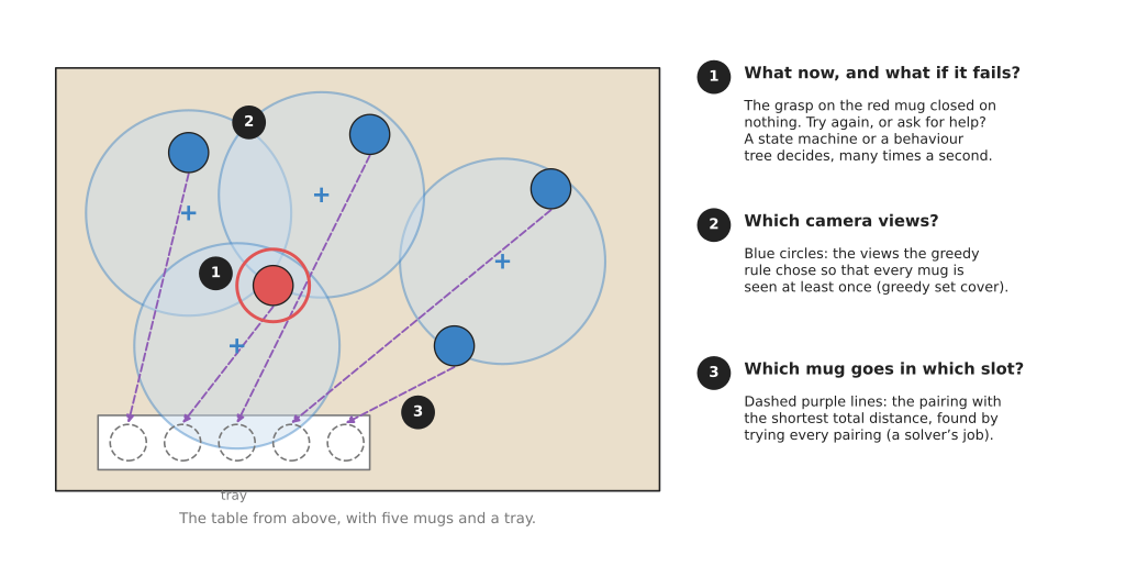
The red mug is the one whose grasp just failed, so a state machine or a behaviour tree decides to try again. The blue circles are the four camera views that a greedy rule chose, out of six, so that every mug is seen. While those views are chosen once, the purple lines do a different job: they pair each mug with a tray slot so that the total distance is the shortest of all 120 pairings, which the script found by trying every one.
3. The four techniques#
Each of the four techniques has its own page, and they split into the two kinds of question above. While the first two react to events as they happen, the last two choose the best set or the best order.
- Finite state machines describe the task as a small set of named situations, such as "grasp" or "carry", joined by arrows that say which event moves the robot from one situation to the next.
- Behaviour trees describe the task as a tree of steps and checks. The tree is re-checked many times a second, and each part answers "success", "failure" or "still running", so retries and fallbacks are part of its shape rather than extra code.
- Greedy algorithms and set cover build an answer one choice at a time, always taking the choice that looks best right now. A common use is choosing the fewest camera views that together see every object.
- Optimisation solvers search for the best answer to a problem written as numbers, a goal and rules. They order picks, assign objects to places and pack boxes, using libraries such as Google's OR-Tools.
Most used, and also used#
The pages of this chapter are in two groups, and the group a page is in tells you how likely you are to need it. The first group, most used, holds finite state machines and behaviour trees. Nearly every arm program has one of the two, because every task has steps, retries and failures to handle. The second group, also used, holds greedy algorithms and set cover and optimisation solvers. You need them only when a task has many choices to put in order, such as which views to take or which part goes in which pocket, and many arm programs never have that problem.
4. How they compare#
Since each technique was described on its own above, the table below now sets the four side by side. Read each row as one technique, and read the columns as the question it answers, how often it runs, what it needs as input, and what it gives back.
| Technique | Question it answers | How often it runs | What goes in | What comes out |
|---|---|---|---|---|
| Finite state machine | What do I do now, given what just happened? | All the time, on every event | The current state and the latest event | The next state, and the action it starts |
| Behaviour tree | What do I do now, and what if it fails? | All the time, often 10 to 100 times a second | The world as the checks see it | The step to run now, and success, failure or running |
| Greedy algorithm | Which small set of choices covers everything? | Once per task or batch | A list of choices and what each one covers | A set of choices, usually close to the smallest |
| Optimisation solver | What is the best order or assignment? | Once per task or batch | Numbers, a goal and rules | The best answer it can prove, or the best it found in time |
Because the first two rows decide which step runs, they are about control flow, while the last two rows are about choice, because they decide what those steps work on. This means a real robot program uses both kinds together, so that a behaviour tree runs the task and one of its steps calls a greedy rule or a solver.
5. When each one runs#
The table above has a column for how often each technique runs, and that difference in timing is easiest to see on a single real run. The picture below comes from the state machine on the finite state machines page, which moves two mugs to a bin and whose first grasp closes on nothing.
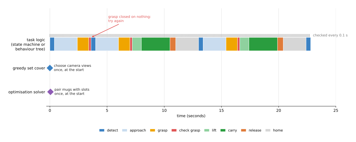
The coloured bar is the state that the task logic was in at each moment, and the small ticks above it show that this state is checked every tenth of a second. Below that, the two diamonds are single calls made once at the start, where one chooses the camera views and the other pairs mugs with tray slots.
This timing decides how fast each technique has to be. Because task logic runs thousands of times in one task, each check must take well under a millisecond. A chooser, however, runs only once, so it can take a few hundred milliseconds, or even seconds, if that buys a better answer.
6. How this chapter connects to the others#
Because task logic decides which step runs rather than doing the work of the step itself, the techniques here sit on top of every other chapter of this book. This means each step in a state machine or a behaviour tree calls something from one of those chapters.
- The "detect mug" step uses the image and point cloud processing chapter to cut the mug out of the picture, and the geometry and cameras chapter to turn its pixels into a position.
- The "is it the same mug as before?" check uses the searching and matching chapter.
- The "move above mug" step calls the planning and search chapter to find a path, and the control and motion chapter to follow it.
- A "holding mug?" check often reads a steady gripper width or force from the fitting and estimation chapter.
Learned models meet this chapter in two places as well. First, a learned model can be one step inside the tree, in the place where a programmed step would otherwise sit. A detector from Book 7's object detection page can be the "detect mug" step, and a model from collision and failure detection can be the "did the grasp fail?" check. While those models replace a step, the tree around them stays the same.
Second, a language model can sit above the tree instead of inside it. The page language models as planners shows a model that turns a spoken request into a list of steps. Even then, those steps usually run inside a state machine or a behaviour tree, because that part must be fast and must always do the same thing.
The map of the whole book, which shows where this chapter sits among the others, is on the map of techniques.
7. Where to read next#
- Start with finite state machines, because they are the simplest way to write task logic and the next page builds on them.
- Then read behaviour trees, which most robot arm programs use today for the same job.
- Greedy algorithms and set cover and optimisation solvers cover the "which ones, and in what order" questions, which come up once a task has many choices in it.
- Book 3 shows behaviour trees in real code in behaviour trees: putting a task in order, and compares state machines and behaviour trees in scripted logic.
8. Using it in Python#
Section 4 said that a real program uses both kinds of technique together, so that the task logic runs the job while one of its steps calls a chooser, and section 5 showed the difference in timing between the two. This section puts that sentence into Python. After reading it you will have seen a solver called once and a behaviour tree ticked many times, in the same file, and you will know which of those lines a library wrote for you.
The example empties a table of three mugs into three tray slots. SciPy chooses which mug
goes in which slot, and py_trees carries the answer out.
import numpy as np, py_trees
from scipy.optimize import linear_sum_assignment

# The chooser runs once: pair mugs with slots so the total travel is smallest.
cost = np.array([[0.32, 0.55, 0.41],      # cost[mug][slot], in metres of travel
                 [0.60, 0.28, 0.37],
                 [0.44, 0.39, 0.25]])
mugs, slots = linear_sum_assignment(cost)
plan = list(zip(mugs, slots))

# The task logic runs many times a second and works through that plan.
class PlaceMug(py_trees.behaviour.Behaviour):
    def __init__(self, mug, slot):
        super().__init__(name=f"mug {mug} to slot {slot}")
        self.mug, self.slot = mug, slot

    def update(self):                     # called on every tick while this step is active
        if grasp_failed(self.mug):
            return py_trees.common.Status.FAILURE
        if placed(self.mug, self.slot):
            return py_trees.common.Status.SUCCESS
        return py_trees.common.Status.RUNNING

root = py_trees.composites.Sequence(name="empty the table", memory=True)
root.add_children([PlaceMug(m, s) for m, s in plan])
tree = py_trees.trees.BehaviourTree(root)

while root.status != py_trees.common.Status.SUCCESS:
    tree.tick()                           # one pass over the tree
    sleep_until_next_tick()
For the costs above the solver pairs mug 0 with slot 0, mug 1 with slot 1 and mug 2 with
slot 2, for a total of 0.85 metres. The two halves of the file run at completely
different rates, which is the point section 5 made: linear_sum_assignment is called
once and returns in well under a millisecond here, while tree.tick() runs perhaps ten
to a hundred times a second for as long as the task lasts.
What the libraries do for you is narrow and worth naming. SciPy's
linear_sum_assignment finds the best pairing exactly, not approximately, so you do not
write a search. py_trees gives you the tick, the three answers, and the composite
nodes that combine them, so you do not write the engine that decides which step is
active.
What you still write is the work itself. grasp_failed, placed and
sleep_until_next_tick are your functions, and so is every leaf of the tree, because a
behaviour tree library has no idea what a mug is. Building the cost matrix is yours too,
and that is usually the harder half of using a solver, because the numbers have to come
from somewhere real.
What you have to decide or measure is the cost numbers and the tick rate. A cost of 0.32 metres is a claim about your cell, and if you guess it the solver will confidently return the best answer to the wrong question. The tick rate has to be fast enough that the tree notices a failure before it matters and slow enough that the checks inside it finish, which section 5 puts at well under a millisecond of work per tick. Whether the plan is recomputed after every mug is your decision as well, because a mug that slipped may have changed the costs.