The techniques in this book look very different from each other at first. One turns a pixel into a position, another finds a path round a table, and another keeps a motor at the right angle. However, almost all of them are built from the same six ingredients, so this page explains those six ingredients one at a time, with a small example of each on a robot arm.
It is for a reader who has read programmed, not learned and has never studied algorithms. Once you know the six ingredients, each later technique page reads as a new way of putting familiar pieces together.
The six ingredients are these, and each of them gets its own section below:
- frames and transforms, for saying where things are;
- arrays and grids, for holding many numbers in order;
- graphs, for places and the ways between them;
- noise and uncertainty, for the fact that every sensor is a little wrong;
- cost functions, for saying which answer is best;
- loops that run at a fixed rate, for doing the same work many times a second.
Contents#
- Frames and transforms
- Arrays and grids
- Graphs
- Noise and uncertainty
- Cost functions
- Loops that run at a rate
- Where each building block appears in this book
- Where to read next
- Using it in Python
1. Frames and transforms#
The first ingredient answers the question of where a thing is, because a position is always measured from somewhere. So "the mug is 300 mm away" means nothing until you say 300 mm from what, and in which direction.
A frame is that "from what", and it is a starting point, called the origin, together with a set of directions, called the axes. Each axis is a direction in which you measure, so on a flat table there are two axes, x and y, while in space there are three, x, y and z. A frame is always fixed to one physical thing. For example, a robot arm has a base frame fixed to its base, and a camera has a camera frame fixed to the camera. Book 1 introduces frames in position, frames and transforms.
The same mug has different numbers in different frames, because the camera measures the mug from the camera while the arm needs to know where the mug is from the base. So the program must convert the camera's numbers into the base's numbers, and a transform is the recipe for that conversion. For a solid object that does not bend, the transform has two parts. First a rotation turns the directions of one frame to line up with the other, and then a translation shifts the origin from one place to the other.
Here is a small example on a flat table, seen from above. The camera sits at x = 400 mm, y = 100 mm in the base frame, and it is turned by 90 degrees, so its x axis points the same way as the base's y axis. From there the camera sees a mug at camera x = 50 mm, camera y = 120 mm.
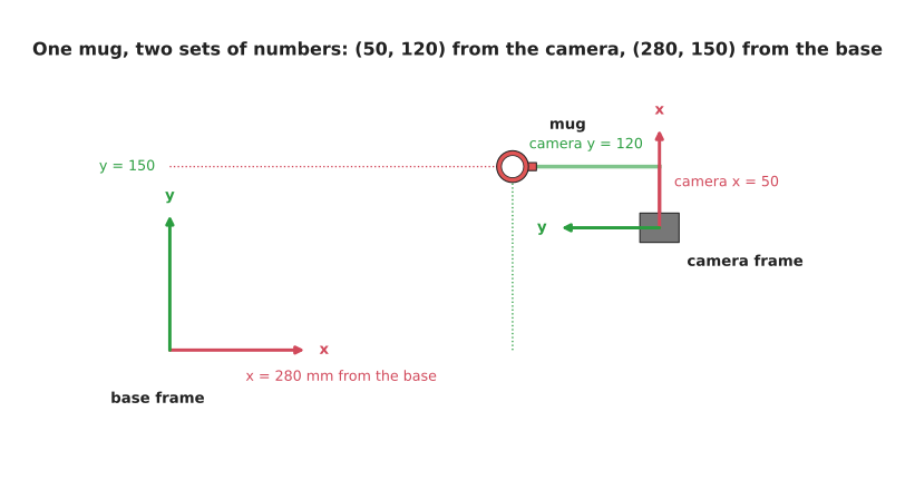
The mug is at (50, 120) when measured along the camera's axes, and at (280, 150) when measured along the base's axes; the red arrows are x axes and the green arrows are y axes.
The conversion goes in two steps, in this order:
- Rotate. Turning the camera's numbers by 90 degrees uses the rule new x = cos(90°) × 50 − sin(90°) × 120, and new y = sin(90°) × 50 + cos(90°) × 120. Since cos(90°) is 0 and sin(90°) is 1, this gives new x = −120 and new y = 50.
- Translate. Add the camera's position in the base frame. That gives x = 400 + (−120) = 280, and y = 100 + 50 = 150.
So the mug is at (280, 150) in the base frame, which you can check against the picture. Real arms do the same thing in three dimensions, with three numbers instead of two. Programs usually pack the rotation and the translation into one 4 by 4 table of numbers, called a homogeneous transform matrix, so that one multiplication does both steps. That matrix is explained on the rigid transforms page.
Transforms can also be chained. For example, if you know the camera from the wrist, and the wrist from the base, you can combine them to get the camera from the base. An arm program does this all the time, and getting one link in the chain wrong is one of the most common bugs in robotics. That is why Book 3 spends a whole page on it: frames, conventions, and the bug class that comes from mixing them.
2. Arrays and grids#
Frames say where a thing is, but a program also needs somewhere to keep many numbers at once, and that is the second ingredient. An array is a list of numbers kept in a fixed order, and each number has a position in the list, called its index. Most programming languages count the index from 0, so the first number is number 0. For example, the row of 16 depth readings on the previous page was an array with indexes 0 to 15.
A grid is an array with rows and columns, like a spreadsheet, so you find one number in it by giving its row and its column. A picture from a camera is a grid in which each cell is a pixel. A picture 640 pixels wide and 480 pixels tall is therefore a grid of 480 rows and 640 columns, which is 307,200 pixels. A colour picture holds three numbers per pixel, which are red, green and blue, while a depth picture holds one number per pixel, which is the distance in millimetres.
The left side of the picture below is a very small depth picture, 6 rows by 8 columns, taken from above a mug.
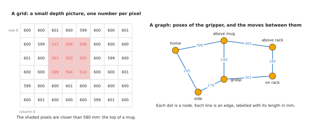
On the left, most cells read about 600 mm, which is the table, and the nine shaded cells read between 503 and 512 mm, which is the top of a mug; the right side is a graph, explained in the next section.
A computer works through a grid in order: row 0 from left to right, then row 1, and so on. Many techniques in this book are therefore loops over a grid. The depth rule on the previous page is one such loop, because it visits each cell and compares its number with 580, and on this grid it marks 9 cells.
A point cloud is also an array, because it is a list of points in which each point has three numbers, x, y and z. So you can think of it as a grid with one row per point and three columns. A depth camera with 307,200 pixels gives up to 307,200 points, one for each pixel that got a reading.
Grids are also used for space itself. For example, a planner can split the table top into small squares and mark each square as free or full, which is called an occupancy grid. The graph search page then finds paths across such a grid.
Arrays matter for a practical reason too, because libraries such as NumPy in Python and Eigen in C++ can do the same sum on every cell of a large array very quickly. Book 1 introduces this in NumPy intro.
3. Graphs#
Arrays and grids hold numbers in rows and columns, but some problems are instead about places and the ways between them, which is the third ingredient. In this book, a graph is not a chart, but a set of places together with the connections between them.
- Each place is called a node. A node can be a pose of the gripper, a square of an occupancy grid, or a state of a task, such as "holding a mug".
- Each connection is called an edge. An edge says you can go directly from one node to another.
- An edge can carry a number, called its weight or its cost. It often means distance or time.
The right side of the picture above is a graph, and its six nodes are poses of the gripper: "home", "above mug", "grasp", "side", "above rack" and "on rack". The lines are moves the arm can make safely, and each line is labelled with its length in millimetres.
A question you can ask of a graph is: what is the shortest way from one node to another? From "home" to "on rack" there are three routes in this graph, so you add the lengths along each one:
- home, above mug, above rack, on rack: 306 + 303 + 180 = 789 mm;
- home, above mug, grasp, on rack: 306 + 240 + 301 = 847 mm;
- home, side, grasp, on rack: 295 + 179 + 301 = 775 mm.
The third route is the shortest, at 775 mm. With six nodes you can check every route by hand, but a real planning graph can have millions of nodes. So the techniques on the graph search page find the shortest route without trying every one.
Graphs appear in many places on a robot arm. For example, a grid of squares is a graph in which each square is joined to its neighbours, and a roadmap is a graph of arm poses known to be free of collisions, used by sampling-based planning. A behaviour tree is another special kind of graph, one that holds the order of a task.
4. Noise and uncertainty#
The first three ingredients all assumed that the numbers are correct, but on a real arm they never quite are. Every sensor is a little wrong, and the error changes each time you read it, so this changing error has a name of its own, noise.
Here is an example. A depth camera looks at a mug that does not move, and the program reads the distance to that mug 20 times in a row.
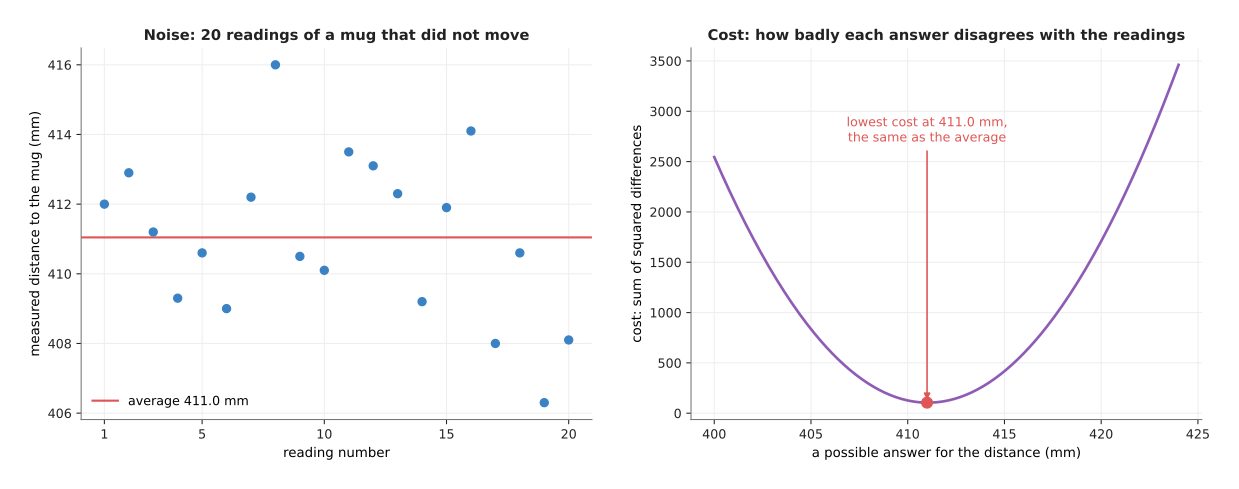
On the left, the 20 readings of the same still mug fall between 406.3 mm and 416.0 mm, around an average of about 411.0 mm; the right side is a cost curve, explained in the next section.
The mug did not move, yet the readings differ by up to 9.7 mm, so no single reading is the truth. The best you can say is that the mug is probably near 411 mm, give or take a few millimetres, and that "give or take" is the uncertainty. For these readings, 16 of the 20 fall within 3 mm of the average.
Noise is not the only kind of error. Sometimes a reading is completely wrong, for example when light bounces off a shiny surface, and a reading like that is called an outlier. Outliers need different handling from ordinary noise, because one outlier can pull an average far away from the truth. Choosing a technique shows this with a picture.
Three chapters of this book exist mostly because of noise and outliers. Fitting and estimation gets a clean shape or a steady number out of many noisy readings. Then the Kalman filter combines each new reading with what it already knew, while random sample consensus (RANSAC) ignores outliers. Every technique page also has a section on what goes wrong, which is very often about noise.
5. Cost functions#
Because noise makes many answers possible, a technique needs a way to pick between them, and that is the fifth ingredient. Many techniques have to choose the best answer from many possible answers, and to do that they need a way to say how good each answer is, as a single number.
A cost function is that way, because it takes one possible answer and gives back one number, called its cost. A smaller cost means a better answer, so the technique's job becomes finding the answer with the smallest cost, which is called minimising the cost. Some techniques use the opposite, a score to make as large as possible, but the idea is the same.
Here is a cost function for the 20 noisy readings above, where the question is which single number best describes the distance to the mug. Take any possible answer, and subtract it from each reading. Then square each difference, so that a reading below and a reading above count the same way, and add up the 20 squares. That total is the cost of that answer, and it is called the sum of squared differences.
The table below shows the cost of four possible answers. Read it top to bottom: the cost falls, reaches its lowest value near the average, and rises again.
| Possible answer (mm) | Cost (sum of squared differences) |
|---|---|
| 405.0 | 835.7 |
| 410.0 | 126.7 |
| 411.0 | 104.9 |
| 415.0 | 417.7 |
The right side of the picture in section 4 draws this cost for every possible answer from 400 to 424 mm. The curve is shaped like a bowl, and its lowest point is at 411.0 mm, which is the same as the average. That is not an accident, because for the sum of squared differences the lowest point is always at the average. This is the simplest case of least squares, which the least-squares fitting page uses to fit lines and planes.
Because a cost function turns a choice into a single number, it appears all through this book:
- In graph search, the cost of a route is the sum of its edge lengths.
- In trajectory optimisation, the cost of a path adds up its length, its jerkiness and how close it comes to obstacles.
- In assignment and matching, the cost of matching two detections is how far apart they are.
- In numerical inverse kinematics, the cost is how far the gripper is from where you want it.
When a technique gives a strange answer, the cost function is often the first thing to check. The technique did find the answer with the lowest cost, so if that answer is wrong, the cost function may be measuring the wrong thing.
6. Loops that run at a rate#
A cost function says which answer is best, but a robot arm does not answer a question once and then stop. It answers the same question again and again, as fast as new readings arrive, because the camera keeps sending new pictures and the joints keep reporting new angles. So the program must use each new reading before the next one arrives.
A loop is a set of steps that repeats, and a loop that runs at a rate repeats on a fixed clock, for example 1,000 times a second. The rate is measured in hertz (Hz), which means "times per second". So 1,000 Hz is 1,000 times a second, which works out as once every 1 millisecond.
Here is the loop that holds one joint at its target angle, in pseudocode:
every 1 millisecond:
    angle   = read the joint's angle sensor
    error   = target angle - angle
    command = a push that grows with the error
    send command to the joint's motor
This is the shape of proportional-integral-derivative (PID) control, which explains how to work out the push.
Each loop gives the technique inside it a time budget. At 1,000 Hz, all four steps must finish in less than 1 millisecond, because if they take longer the next reading is late and the arm stops moving smoothly. A camera loop at 30 Hz, in contrast, has about 33 milliseconds per picture. So a technique that is fine in the camera loop can be far too slow for the joint loop.
Different parts of an arm run at different rates. A joint controller often runs at 500 or 1,000 Hz, while a camera runs at 15 to 60 Hz. A planner may run only once before each move, and the "decide what to do next" logic may run only when something changes. Choosing a technique draws these budgets side by side.
7. Where each building block appears in this book#
Now that all six building blocks have been described, the table below shows where each of them matters most. Read each row as one block, with the chapters in which it does most of the work.
| Building block | Main chapters | One example |
|---|---|---|
| Frames and transforms | geometry and cameras, planning and search | turning the mug's camera position into a base position |
| Arrays and grids | image and point cloud processing, searching and matching | marking every depth pixel closer than 580 mm |
| Graphs | planning and search, decisions and task logic | the shortest route from "home" to "on rack" |
| Noise and uncertainty | fitting and estimation, geometry and cameras | 20 readings of one still mug |
| Cost functions | fitting and estimation, planning and search, decisions and task logic | the sum of squared differences |
| Loops at a rate | control and motion, fitting and estimation | the 1,000 Hz joint loop |
Learned models in Book 6 use the same building blocks. A model's input is an array, and its training minimises a cost function, which Book 6 calls a loss. A trained model then runs inside a loop at a rate, as running a model on a robot describes.
8. Where to read next#
- Choosing a technique is the next page. It uses these building blocks to compare techniques.
- Vectors and matrices for a robot arm in Book 1 explains the maths behind rotations and translations.
- Rigid transforms takes section 1 into three dimensions.
- How a model learns in Book 6 shows a cost function being used to train a model.
9. Using it in Python#
The six sections above described the six ingredients with arithmetic and pictures, and section 7 said which chapters use each one. This section shows two of the six as real Python, so that you can see what they look like in a file. The two are frames and transforms from section 1 and cost functions from section 5, because those are the two you meet first in any arm program, and both are one library call rather than a page of code.
The libraries are SciPy, whose Rotation class converts between the different
ways of writing a turn, and NumPy, which does the matrix multiplication and the
whole-array arithmetic. The numbers below are the camera-to-base example from
section 1, so the answer should be the mug at (280, 150).
import numpy as np
from scipy.spatial.transform import Rotation

# Ingredient 1: the camera's frame in the base frame, packed into one 4 x 4 matrix.
T_base_camera = np.eye(4)
T_base_camera[:3, :3] = Rotation.from_euler("z", 90, degrees=True).as_matrix()
T_base_camera[:3, 3] = [400.0, 100.0, 0.0]        # millimetres

mug_camera = np.array([50.0, 120.0, 0.0, 1.0])   # the trailing 1.0 applies the shift
mug_base = T_base_camera @ mug_camera
print(mug_base[:3])                               # [280. 150.   0.]

# Ingredient 5: the cost of one possible answer, over the 20 noisy readings.
readings = np.loadtxt("mug_distances_mm.txt")     # 20 numbers

def cost(answer):
    return np.sum((readings - answer) ** 2)       # sum of squared differences
The libraries do two things for you here. SciPy turns 90 degrees about the z axis
into the nine numbers of a rotation matrix, and it will just as happily read that
turn back out as a quaternion or as three angles, which saves you writing sines
and cosines and getting a sign wrong. NumPy then applies the 4 by 4 matrix with a
single @, and subtracts one number from all 20 readings without a loop.
What you still write yourself is the bookkeeping, and it is the part that goes
wrong. Nothing in NumPy knows that T_base_camera means "the camera's frame
expressed in the base frame" rather than the other way round, so if you build it
backwards the code runs and gives a plausible wrong answer. The same is true of
the order when two transforms are joined, and of the cost function, because
cost is your definition of what "best" means and the technique will faithfully
find the smallest value of whatever you wrote.
What you have to decide or measure is where the camera actually is. The 400, the 100 and the 90 degrees in that code came from a measurement, and calibration is the technique that makes them accurate, because an error of one degree in the angle costs about 6 mm at a third of a metre. For the cost function you have to decide whether squaring is right at all, since squaring makes one wild reading count a hundred times more than a reading 10 times closer, which is exactly the outlier problem section 4 described.
The other four ingredients also come ready-made, and each one is named on the page that uses it: the graph search page for graphs, the Kalman filter page for noise and uncertainty, and the PID control page for loops that run at a rate.