This page gives the results of this solution and explains them. It gives the scores in the two kinds of arrangement, says why the solution failed, and places it beside the other five. The examiner marked every number on it.
Contents#
- The results in the two kinds of arrangement
- Why it failed: the names it reached for
- Where it is strong and where it breaks
- The general ideas behind this
- Where it sits among the other five
- What it costs to run, and the licence
1. The results in the two kinds of arrangement#
The examiner marks every solution on spaced and on crowded arrangements, as the examiner explains. Each kind is five blocks of 20 held-out arrangements.
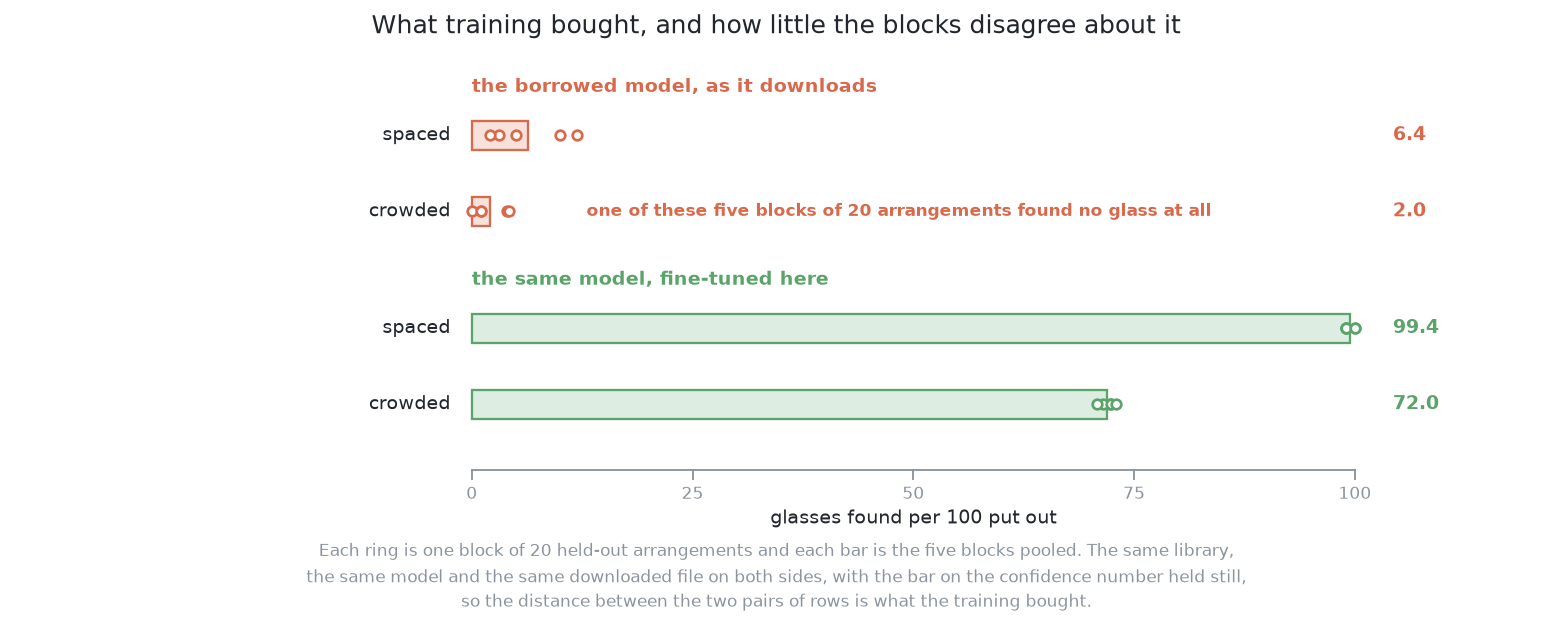
This solution found 6.4 glasses in every 100 when they were spaced, and 2.1 when they were crowded. Both are the worst scores in the book by a wide margin. They also vary the most from block to block. The five spaced blocks run from 2.0 to 11.9 per 100. The five crowded blocks run from 0.0 to 4.2. One whole crowded block found no glass at all. The spread does not change the conclusion. Its best block is still far below the worst block of any other solution. The results puts these scores beside the other five.
For a single picture, the usual result is nothing. Each block is 20 arrangements
seen from three stations, so 60 pictures. The model named no drinking vessel in
49 to 58 of the 60 spaced pictures, and in 56 to 60 of the 60 crowded ones. For
such a picture, Finder.find returns an empty list. The examiner then marks
every glass on the table as missed.
What it did report was right. No glass was merged, split or falsely reported, in any block. A merge is two glasses reported as one. A split is one glass reported as two. So this solution fails by saying nothing, not by inventing glasses. This kind of failure is harder to notice. A method that reports no glass looks the same as an empty table.
The masks it kept were mostly good. It found 12 glasses of the two kinds with a stem, and 20 of the two kinds without one. On glasses without a stem, the block medians cover 99.8 to 100.0 per cent of the glass. On glasses with a stem they cover 44 to 79 per cent. A stem is thin, and the model builds its outline from a few coarse patterns that cannot show thin parts. At the median, 3.3 per cent of a kept mask was not the glass. The rule written by hand had 0.0. This is because the outline is enlarged to the size of the picture and comes out a little too big.
So the model outlines well when it gives an outline at all. The next section asks why it so rarely gave one.
2. Why it failed: the names it reached for#
The results above show a model that is almost always silent. This section uses
one more measurement to find out why.
what_it_named.py
runs the model on 36 held-out pictures with no name filter. It prints every name
the model gives. Over those 36 pictures the model returned 87 named objects.
Only 5 had a name the filter accepts.
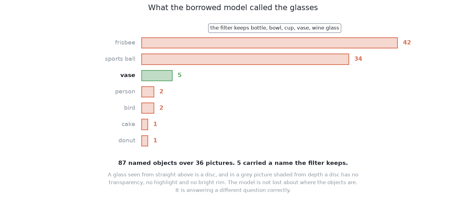
The model is not blind. It finds the glasses, but it calls them sports balls and frisbees. A glass seen from straight above is a disc. The nearest round things on the model's list are a ball and a frisbee.
The cause is a domain gap. A domain gap is the difference between the data a model was trained on and the data it is used on. Here the gap has two parts.
- The picture is not a photograph. The cell gives a grey picture, shaded by how far away each surface is. A model trained on photographs relies on real light: shading on curved surfaces, shadows, and colour. Very little of that is in these pictures.
- The glasses do not look like glasses in photographs. In a photograph, a model sees that an object is clear, with a bright highlight on the side and the rim. This cell draws its glasses as solid shapes. Only the outline is left.
One fix is possible, and it is refused. Adding "sports ball" and "frisbee" to the list would raise the score at once. But that means choosing the filter after looking at the answers on this cell's own data. This solution exists to avoid exactly that. Measuring the names is allowed. Acting on them is not.
The confidence cut-off played no part in this failure. The lost outlines were dropped because of their names, before the cut-off was checked.
Now that the cause is known, the next section weighs what the solution does well against where it breaks.
3. Where it is strong and where it breaks#
The section above found the cause of the failure. This section sets it beside the solution's strengths. All of them come from one fact: nothing is fitted.
There is nothing to collect, train or keep up to date. So this solution was tried in an afternoon. It showed what a borrowed model is worth before anybody spent time on labels. It also deals with the merge directly, because the model gives one outline per object, not one per joined shape. It needs no graphics card of its own. No other solution can be cheaper. If this one had been good enough, several others would not be needed.
The weaknesses are of two kinds: what the borrowing costs, and what it cannot do.
The borrowing costs the naming, and the naming decided the score. The names it reached for shows this. The other two costs are small. The outline is built coarsely and then enlarged, so each width has an error that does not average out. The confidence is not a probability here, so the cut-off is a setting chosen by hand, as what it is explains.
It cannot do anything that needs training. Its outlines cover only pixels the camera saw. So a glass partly behind another one is read as a smaller glass in the wrong place. A fully hidden glass leaves no pixel at all, so no model can find it. Looking again at what was hidden gives the shared answer to that.
So this is the first thing to run, not the thing to put in a finished product. Its value is the comparison it makes possible. The next section names the general ideas behind this result, because they apply outside this cell too.
4. The general ideas behind this#
The strengths and weaknesses above each come from a general idea. This section gives four of them, and says when each one is the wrong choice.
Zero-shot transfer — using a model on a task it was never fitted for#
A model is used zero-shot when it gets no examples of the new task at all. It relies only on what it learned before. This works when the new task is really a special case of the old one. Here it seemed true, because the model's training data contains drinking vessels on tables. It was not true, because these pictures are not photographs. So "the same objects" is not enough. The inputs must also be the same kind of input.
Zero-shot is usually a good first try when a general model exists and labels are expensive. It takes an afternoon and shows how hard the problem is. It is usually wrong as a final answer when the input looks different from the training data. It is also wrong when you need finer categories than the model knows. Both are true here.
Closed-vocabulary detection — a fixed list of things that can be named#
This model can only give names from a list that was fixed when it was trained. This is called a closed vocabulary. So the names here can only filter. The list cannot contain this cell's four kinds of glass, because it was written without this cell. It also explains the failure. The model has no way to say "a round thing I do not know", so it says "sports ball".
A closed vocabulary is good when your categories are on the list. Then it is fast and predictable. When they are not on the list, there are two usual fixes. One is to train the model further on your own categories, which is solution 4. The other is a model that takes a description in words instead of a fixed list. That removes the limit, but its outlines are much less reliable.
One-stage detect-and-segment, against propose-then-classify#
This model finds and names objects in one pass. Solution 5 does it in two steps instead. One model proposes regions, and a second part decides which to keep.
One pass is faster and simpler. It is the right choice when the model already knows the categories you want. Two steps are better when it does not. This is because finding a shape works across a domain gap much better than naming does. A shape is a shape everywhere. But what counts as a cup was learned from somebody else's data. This cell shows that split clearly. The finding part of this model works. The naming part failed.
Calibration under changed input#
A model's confidence is calibrated when it is right about as often as it says. For example, outlines with confidence 0.6 are right about 60 times in 100. A model gets this calibration from the data it was trained and checked on. On different data the calibration breaks. The order of the scores often still works.
Trusting the order is usually safe, and this solution does only that. Trusting the numbers needs a fix. The fix is a small correction fitted on data where the answer is known. It is cheap and usually worth doing before a cut-off decides anything important. This solution leaves it out, because its whole point is to fit nothing.
These four ideas put this solution at one end of a range. The next section lays out that range across the six solutions.
5. Where it sits among the other five#
The ideas above are about how much each solution fits in the cell. This section uses that to put the six in order.
- At this end, nothing is fitted. The borrowed model's own names pick the glasses.
- Solution 5 borrows a model that outlines without naming. It trains a small keeper here to choose the glasses. So it replaces the part that fails worst.
- Solution 4 trains this same model further on this cell's pictures. Solution 6 does the same with a different kind of model.
- Solution 2 trains everything here and borrows nothing.
- Solution 1 is outside this range. It has no model and fits nothing.
Read in this order, the six solutions show what each extra step of fitting gains. This solution is the baseline.
Solution 4 gives the clearest comparison. It is this same model with the same starting weights, trained further on this cell's pictures. Only the training differs, so the gap between the two shows what training gained. The same model, fine-tuned explains why this pair is so clean.
The picture below shows the gap. Each mark is one block of 20 held-out arrangements. The spread of one solution's marks shows how much its score changes between blocks. The distance between the two groups shows what the training gained.
This comparison is only cheap because this solution costs almost nothing to run. The last section gives that cost.
6. What it costs to run, and the licence#
The comparison above needs this solution to be cheap. This section gives its cost, and the one condition that comes with the weights.
It needs the Ultralytics package and the model's weights. The package downloads the weights by itself on first use. The download is 6.4 MB and is not committed. It runs on this machine's built-in graphics through PyTorch's MPS backend. MPS is how PyTorch uses the graphics on an Apple machine. One picture takes 0.02 seconds once the model is loaded. A whole block of 60 pictures takes about six seconds, with the rendering. It needs no labelled pictures, no training and no weights file to keep up to date.
The real cost is the licence. Ultralytics YOLO26-seg uses the AGPL-3.0 licence (GNU Affero General Public License, version 3). The AGPL has one important rule. Anybody who shares the software, or offers what it does over a network, must publish their full source code under the same licence. That network rule covers a product that never ships the model and only sends its answers to users. Everything else in this project uses permissive licences, which have no such rule. So this one part would change the terms of the whole perception step in a product.
For these six solutions the licence costs nothing, because nothing is shipped or served. The design also does not depend on this particular model. Solution 6 already uses a segmenter with a permissive licence. So for commercial work, the model could be replaced easily.
The next chapter is solution 4. It keeps this model and its licence, and adds the training this solution refused. It shows how much of the gap training closes.