This page answers one question: how can a robot tell that an object in its fingers is starting to slide out, early enough to do something about it? To answer that, it explains the force signals a model reads, how a slip model works and is trained, the models people have published, and why this job is harder than it looks.
It is written for a reader who has already read touch sensing models, because this page uses the moving dots from its section 4.3. You should also know from how a model learns what it means to train a model on examples.
Before this page, it helps to have read sensor streams, which explains windows of readings, smoothing, rates of change and thresholds that do not flicker. A slip model reads the same kind of window.
Contents#
- What it is
- What goes in and what comes out
- What slip looks like in the signal
- How it works inside
- How it is trained
- Well-known models
- Where this is going
- Where to read next
1. What it is#
A slip model reads the force signals from a gripper over a short stretch of time and says whether the held object is starting to slide.
Here is an everyday example of the same skill in a person. You carry a full glass of water, and your hand is a little wet. You feel a tiny slide on your fingertips before the glass moves far, so without thinking you squeeze a bit harder, and the glass stays put. In other words, you did not wait to see it fall.
So a slip model tries to give a robot that same early warning. The word slip means that the object moves relative to the fingers, and the useful moment to catch it is the very start, which is called incipient slip. "Incipient" means just beginning, and at that moment squeezing a little harder still works. However, a second later the object is already on the floor.
This page also covers the wider family of force models, which do a related job. These read force signals and say something else about the contact, such as how the object is sitting in the fingers, or whether a part has clicked into place. However, slip is the most common job, so the page uses it as the main example.
2. What goes in and what comes out#
Now that slip has a name, here is what the model actually reads. The input is a short window of recent sensor readings, where a window means the last few tenths of a second of readings, taken together. Those readings can come from several different sensors:
- A tactile sensor on the finger pad, as a short run of tactile pictures, or the positions of the printed dots in each picture.
- A force sensor on the finger pad, giving the push straight in and the push sideways at each moment.
- A force-torque sensor at the wrist, giving six numbers at each moment: a push along three directions and a twist about three directions.
- A small vibration sensor, called an accelerometer, near the finger.
Then the output is usually one of two things. The first is a yes-or-no answer, "slipping" or "not slipping", and the second is a number between 0 and 1 that says how likely a slip is. In the second case the program then compares that number with a limit it chooses.
Some force models give other outputs, such as "the grasp will hold" or "the part is seated", but they all work in the same way.
3. What slip looks like in the signal#
The last section said what goes in and out, and this section shows what the signal itself looks like. A slip leaves marks in the signal, and a slip model learns to recognise them, so it is worth seeing those marks first.
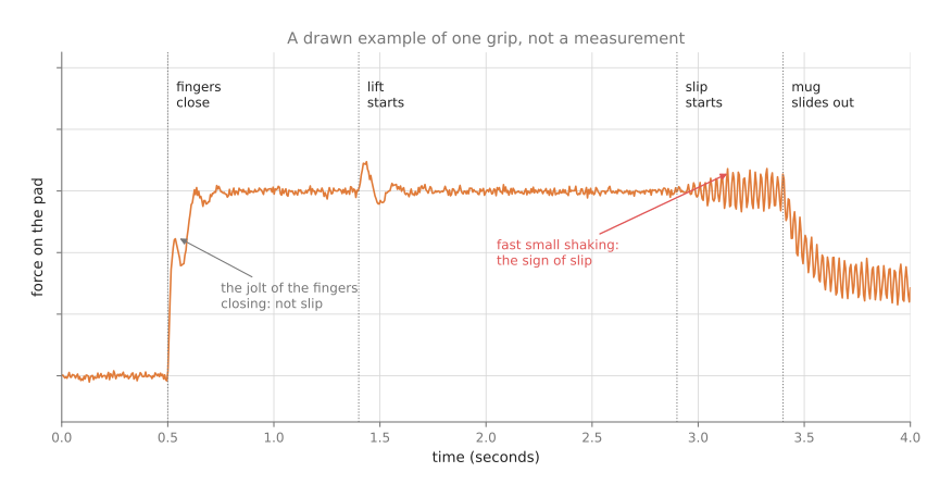
The picture is a drawn example, not a real measurement, and it shows the force on one finger pad during one grip. The force jumps when the fingers close, and it wobbles briefly. Then it wobbles again when the lift starts, and after that it holds steady. When the slip starts, a fast, small shaking appears, and then the force drops as the mug slides out.
However, two things make slip hard to spot by eye, and by a simple rule. The first is that the jolts from closing and lifting look a lot like the shaking from slip, because both are quick changes. So a rule that says "a quick change means slip" fires on every lift. The second is that the drop in force comes late, because by the time the force has clearly dropped, the object is already sliding out.
But a tactile sensor shows slip in a second way, and this one comes earlier.
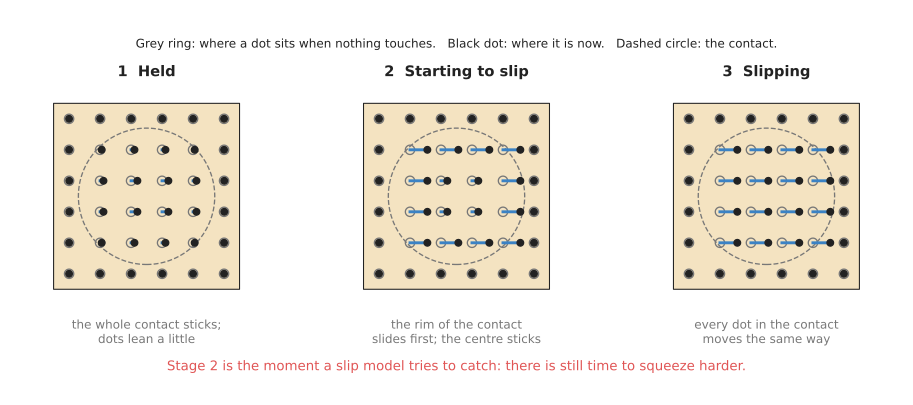
The picture shows the dots on a gel pad at three moments. While the object is held, the dots in the contact lean a little, all together. When slip starts, the dots at the rim of the contact slide first, while the dots in the centre still stick, and the rim goes first because that is where the pressure is lowest. Once the object slips fully, every dot in the contact moves the same way.
Stage 2 is the moment a slip model tries to catch, because the centre still holds and there is still time to squeeze harder.
4. How it works inside#
4.1 One window at a time#
The last section showed what slip looks like, so this section says how a model picks it out. A slip model does not read the whole grip at once. Instead, it reads one short window at a time, and it moves the window forward as new readings arrive.
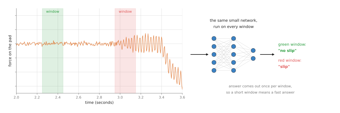
The picture shows two windows on the same signal. The green one covers a steady stretch, so the network says "no slip", while the red one covers the fast shaking, so the network says "slip", and the same network runs on every window.
The steps are these:
- The program keeps the last few tenths of a second of readings in memory.
- It passes that window to the model.
- The model gives back "slip" or "no slip", or a number for how likely a slip is.
- The program acts on the answer, and the window moves on.
The window length is a choice with a cost attached to it. A short window gives an answer sooner, but it holds less evidence, so the model makes more mistakes. Instead, a long window is more reliable, but its answer comes later.
4.2 What kind of network#
The window is the same idea for every sensor, but different signals suit different networks.
For tactile pictures, the model often uses a convolutional neural network (CNN) to read each picture, as in the touch sensing page . A second part then looks at how the pictures change over the window. Then a common choice for that second part is a long short-term memory (LSTM) network. An LSTM is a network that reads a sequence one step at a time and keeps a short memory of what it has read so far.
For a force signal, which is only a few numbers at each moment, a simpler network is often enough, because it can read the window as one list of numbers. Some models first turn the window into a set of frequencies, which shows the fast shaking of slip more clearly. A network of this kind, trained on your own recorded windows, is what section 6.2 recommends.
Two other shapes are common enough that the shortlist later on this page recommends both of them. The first is not a network at all. You reduce each window to a few summary numbers yourself, such as its average and how much it wobbled, and you give those numbers to an ensemble of decision trees, which is what section 6.1 recommends as the first thing to try. The second starts from a model somebody else has already trained on a very large number of unlabelled tactile pictures, and trains only a small part on top of it to answer the slip question. That is what section 6.4 recommends, with Sparsh as the model you start from.
4.3 Joining touch with a camera#
Some models also look at a camera picture of the object in the gripper. The camera can see the object move a lot, while the tactile sensor can feel it move a little, so together they catch more slips than either one alone. The clearest published example of this is Making Sense of Vision and Touch, which learns one set of numbers from a camera picture, the six wrist force-torque numbers and the joint readings at once, and section 6.5 describes it.
5. How it is trained#
The last section described the network, and this section says where its examples come from. A slip model learns from windows of readings that each have the right answer, "slip" or "no slip", and getting those answers is the hard part.
So the usual way is to cause slips on purpose, many times over, and record them. A robot grips an object gently and lifts it, or pulls it sideways, or tilts it, so that some of those grips hold and some slip. For each window, someone then needs to know whether a slip was happening, and people find that out in three ways:
- They watch the object with a camera and a tracking marker. If the object moves relative to the fingers, that window is marked "slip".
- They use the tactile dots. If the dots in the centre of the contact move, the object has slipped.
- They mark it by hand from a video. This is slow and it is done for small sets only.
Published slip data sets are small, and they are much smaller than the data sets for camera models, because every example costs a real grip on a real robot. That is one reason slip models often fail on objects unlike the ones they were trained on.
6. Well-known models#
Touch has fewer models you can download than any other area in this book, and the sensor on your robot decides which of the few you can use at all. So this section is organised by hardware. A force-torque sensor at the wrist, an optical gel sensor such as GelSight Mini or DIGIT, an array of pillars, and a magnetic skin each lead to a different answer, and for most of them the answer is that you train a small model of your own.
Read the table one row at a time. The left column names the method and says whether a
developer starting today would reach for it. The right column holds everything else:
the sensor the method needs, what it is best at, how big the model is, its licence, and
the one case that should make you choose it. A cell says not stated where nobody has
published the figure. Where the licence is yours, the model comes out of your own
training run, so no licence restricts it.
| Model | What decides it |
|---|---|
| 6.1 Features and a tree ensemble, most used in 2026 | It works with any of the sensors above. It is best when you have a few hundred recorded grips. The size is yours to choose, and the licence is yours. Pick it for your first attempt, on any sensor. |
| 6.2 A small network on the raw window, most used in 2026 | It works with any of them, and with tactile pictures too. It is best when you have thousands of recorded grips. The size is yours to choose, and the licence is yours. Pick it when the tree ensemble has stopped improving. |
| 6.3 GelSight's marker tracker, most used in 2026 | It needs a gel with printed dots. It is best at measuring the sideways pull, with no training, and it is not a learned model at all. The licence is GPL-3.0. Pick it when you own such a sensor and want the signal today. |
| 6.4 Sparsh with a force-and-slip head, worth betting on | It needs a DIGIT, a GelSight'17 or a GelSight Mini. It is best at slip and three-axis force from few labels. There is a small backbone and a base one, and their parameter counts are not stated. The licence is CC BY-NC 4.0, with no commercial use. Pick it when you own one of those three, and sell nothing. |
| 6.5 Making Sense of Vision and Touch, historical | It needs a wrist force-torque sensor, a camera and the joint readings. It is best at a contact job with no slip labels at all. Its size is not stated, and its licence is MIT. Pick it when you want the idea and will retrain it. |
6.1 Hand-made features and a tree ensemble#
This is the method most used in 2026, and it is not a published model at all. Size xs, a laptop, and the licence is yours, because the model comes out of your own training run. You turn each window into a short list of summary numbers, and you give that list to an ensemble of decision trees built one after another, each correcting the mistakes of the ones before it. Veiga and colleagues (2015) did this with random forests on a BioTac, a fingertip-shaped sensor filled with fluid, and the shape of the answer has not changed since.
The one idea this method is built on is that the learning never sees the signal. You decide beforehand which properties of a window could possibly matter, you compute them yourself with arithmetic you wrote, and the trained part only has to work out how to combine the handful of numbers you handed it. Those numbers are ones you can say out loud: the average of each axis, how much each axis wobbled, the largest change between two neighbouring readings, and how much of the signal sits in the fast part.
Inside, that leaves nothing at all that reads the window. A window of twenty readings on six axes is 120 numbers, and your own feature function turns those 120 into about two dozen before any learning happens. What learns is a stack of short decision trees. Each tree is a chain of yes-or-no questions, one feature at a time, such as "did the sideways axis wobble by more than this much?", and each new tree is fitted to the error that the trees before it left behind. The network in section 6.2 is wired the other way round. Its first layer is connected to all 120 raw numbers at once, and what training changes there is how those raw numbers are combined, so nobody has to name what matters.
What the idea buys is accuracy from very little data. The trees only choose among features you already computed, so there are far fewer numbers to fit than in a network that has to learn its own front end as well as its answer. It trains in seconds on an ordinary processor, it answers in well under a millisecond, and it will tell you which feature it leaned on, so a failure teaches you something about your sensor rather than nothing. What the idea costs is that a property you did not think to compute is one the model can never see. Your feature list is a guess about the physics of your own gripper, and a wrong guess is invisible, because the model simply stops getting better and does not say why.
On a robot arm the difference shows up on your first day of data collection. A day of deliberate slips buys a few hundred grips, which is perhaps thirty objects in ten poses. Trained on that, this method is usually usable and the network of section 6.2 usually is not, because a few hundred examples give the network enough freedom to memorise the grips it saw rather than learn what a slip looks like. You find that out when the arm grips an object that was not in the set, which is after the mug is already on the floor.
So you would pick this rather than the network in section 6.2 because of how much data you have, and for no other reason. The thing that most often goes wrong here is not the model but the test: if you split the windows at random, two windows one reading apart land on opposite sides of the split, and the high score that follows means nothing.
The library is scikit-learn, whose own COPYING file is the BSD 3-Clause licence. The
class is
HistGradientBoostingClassifier.
import numpy as np
from sklearn.ensemble import HistGradientBoostingClassifier
from sklearn.model_selection import GroupKFold, cross_val_score

# Your own recording, already cut into windows: 20 readings of six wrist numbers
# each, one answer per window, and the number of the grip each window was cut from.
windows = np.load('slip_windows.npy')         # shape (number of windows, 20, 6)
answers = np.load('slip_answers.npy')         # shape (number of windows,), 0 or 1
grips = np.load('slip_grip_numbers.npy')      # shape (number of windows,)

def features(window):                         # one window: 20 readings by 6 axes
    step = np.diff(window, axis=0)            # how much each axis changed each reading
    return np.concatenate([window.mean(0), window.std(0),
                           np.abs(step).max(0), (step ** 2).sum(0)])

x = np.array([features(w) for w in windows])
model = HistGradientBoostingClassifier(max_iter=200)
# GroupKFold splits by grip, not by window, which is the correct split described above.
scores = cross_val_score(model, x, answers, groups=grips, cv=GroupKFold(5))
print('score on each held-back fifth of the grips:', scores)
model.fit(x, answers)                         # then train on everything and save it
scikit-learn builds the trees and scores the model five times over, so max_iter is
the only choice you make. What you supply is the three files, which means causing slips
on purpose and writing down what happened, as section 5 describes. The grip number is
the part people forget to record, and without it the split above is impossible.
6.2 A small network of your own on the raw window#
This is also most used in 2026, by people who have collected thousands of grips, and it is the only choice when the window holds pictures instead of numbers. Size xs and a laptop for a window of wrist numbers; a window of tactile pictures pushes it to size s and wants a big card to train on. The licence is yours, and PyTorch is BSD 3-Clause. The network reads the window itself, with no features in between. For six wrist numbers, two layers with a few dozen numbers in the middle is enough; for tactile pictures, the arrangement is the one in section 4.2, which Li and colleagues introduced in February 2018 and released no code for.
The one idea here is that the model invents its own summary of the window. You hand it the readings and nothing else, and the part that decides which of those readings matter is itself learned rather than written.
Inside, the difference from section 6.1 is where the window gets reduced. In section 6.1 you reduce it, and the trees never see more than the two dozen numbers you computed. Here the reduction is the network's first layer. Each unit in that layer adds up all 120 numbers of the window, with a weight on each one, and training changes those weights. An average is one such weighted sum, with every weight the same, so the network can learn section 6.1's features if they are the useful ones, along with thousands of combinations nobody would have written down. When the window holds pictures rather than numbers, the reducing is done by a convolutional network reading each picture and a long short-term memory network reading the run of them, which is the arrangement in section 4.2.
What that buys is patterns that no single hand-made number can hold. A per-axis average cannot express "the sideways force rose while the straight-in force stayed flat", because it throws away the order of the readings and keeps the axes apart, while a layer connected to the whole window can represent exactly that. What it costs is examples. The network is fitting its own front end as well as its answer, so it wants thousands of grips where the tree ensemble wanted hundreds, and it tells you nothing about which part of the signal it leaned on. It also costs time, because a wider network is slower and a longer window delays the answer directly, and the answer that arrives after the mug has gone is worth nothing.
The place this choice decides the outcome is a gel sensor. A gel picture has no short list of hand-made numbers that captures it, so section 6.1 has nothing to compute from it, and the early slip signal of section 3, where the rim of the contact slides while the centre still sticks, is a pattern spread across the picture rather than one quantity. With a gel sensor section 6.1 is not the weaker choice; it is not a choice.
So you would pick this rather than the tree ensemble in section 6.1 once your training set runs into the thousands, and you have no choice at all once the window holds pictures. Both the network's width and the window's length have to be timed on the computer that will sit next to the arm, because neither cost shows up in the score.
The library is PyTorch. This is the half that runs while the arm carries the mug.
import collections

import numpy as np
import torch
from torch import nn

# The network you trained, rebuilt so the saved numbers fit into it.
net = nn.Sequential(nn.Linear(6 * 20, 32), nn.ReLU(), nn.Linear(32, 1))
net.load_state_dict(torch.load('slip_model.pt'))
net.eval()                               # switch off the parts that only train

window = collections.deque(maxlen=20)    # keeps only the last 20 readings
slipping = False

while carrying:
    window.append(read_wrist_force())    # your own driver, giving six numbers
    if len(window) < window.maxlen:
        continue
    # Transposed, because training laid each window out one sensor at a time, and
    # the same numbers in a different order are a different input to the network.
    x = torch.tensor(np.array(window).T.reshape(1, -1), dtype=torch.float32)
    with torch.inference_mode():         # nothing is learned here, so keep no gradients
        chance = torch.sigmoid(net(x)).item()
    # Two limits rather than one: the flag turns on above 0.8 and only turns off
    # again below 0.4, so it does not flicker while the number sits near a limit.
    slipping = chance > 0.4 if slipping else chance > 0.8
    if slipping:
        slow_down_and_squeeze_a_little_harder()
net.eval() and torch.inference_mode() between them switch off everything that
belongs to training, and the second also makes each answer faster. torch.sigmoid turns
the raw output into the number between 0 and 1 that section 2 described, and
collections.deque with a maxlen throws the oldest reading away by itself.
What you write yourself is read_wrist_force, which talks to your sensor, and
slow_down_and_squeeze_a_little_harder, which is the response that Book 3's
holding on
page puts in order of cost. You also have to produce slip_model.pt, since there is no
slip model to download. What you decide is the two limits and the window length.
6.3 GelSight's own marker tracker, as the shear signal#
This is most used in 2026 by anyone who owns a gel sensor with printed dots, and it contains no learning at all. Size not stated, because nothing here is trained, a laptop, and GPL-3.0 for the code. It is part of GelSight's own software development kit, gsrobotics. Section 4.3 of the touch sensing page describes what the dots do, and this is the code that measures it.
The one idea is that you can measure the slip rather than predict it. The printed dots are a ruler lying on the gel, and working out where each one went is arithmetic.
Inside, there are no trained numbers at all, and that is the whole difference from sections 6.1 and 6.2. The tracker takes the first picture, finds the dark dots in it and fits them to the grid they were printed in, so every dot gets a name and a starting place. Then, for each dot in each new picture, the Lucas-Kanade method takes the small square of picture around where that dot used to be and searches for the small shift that makes this picture's square look most like the last one's. The answer for one dot is two numbers, how far it moved across and how far down. So what comes out of the whole thing is a field of arrows over the contact, and not the word "slipping". The two learned methods above produce the word and keep no arrows; this produces the arrows and knows no words.
What that buys is the one property neither learned method has. It cannot be confidently wrong about an object it has never gripped, because it is making no claim about objects at all, and it needs no training set, no labels and no retraining when you change the gripper. What it costs is the meaning. The arrows say how far the gel moved, and nothing in them says how far is too far for your gel, your objects and your squeeze, so finding that limit is a set of deliberate slips after all. It is also limited by the camera rather than by the method, because a dot shift smaller than a pixel does not exist in the output.
On an arm, this shows up the first time the gripper holds something that was not in your recordings. A model from section 6.1 or 6.2 answers anyway, and its answer about an unfamiliar object is a guess that comes out looking exactly like a measurement. The dot field has no such failure. That is why the best arrangement is usually not either alone: measure the dot movement here, then feed those two numbers per dot into section 6.1 as features, so the learned part only has to decide what the movement means.
So you would pick this rather than training a slip model on gel pictures, which is section 6.4, whenever you own a gel with dots, because it gives you the signal this afternoon rather than after a data collection campaign. Three costs are about this tool rather than about its size. Its GPL-3.0 licence, read from its own licence file and recorded in the frameworks book's licence table, obliges you to publish the source of anything you link it into. It needs the dots, so a plain gel has nothing to track. And the gel is a consumable, rated by its maker for 1,000 coin presses.
import cv2
import numpy as np
from utilities.gelsightmini import GelSightMini
from utilities.marker_tracker import MarkerTracker

camera = GelSightMini(target_width=320, target_height=240)  # the size in default_config.json
camera.select_device(0)
camera.start()

first = camera.update(dt=0.0)
tracker = MarkerTracker(np.float32(first) / 255.0)   # finds the dots, fits them to a grid
# The tracker reports each dot as (row, column); OpenCV wants (column, row).
start = tracker.initial_marker_center[:, ::-1].astype(np.float32).reshape(-1, 1, 2)
current, previous_grey = start.copy(), cv2.cvtColor(first, cv2.COLOR_RGB2GRAY)

while carrying:
    frame = camera.update(dt=1 / 25)
    grey = cv2.cvtColor(frame, cv2.COLOR_RGB2GRAY)
    moved, found, _ = cv2.calcOpticalFlowPyrLK(previous_grey, grey, current, None,
                                               winSize=(15, 15), maxLevel=2)
    shift = (moved - start)[found[:, 0] == 1]        # each dot's move since the first picture
    print('average dot movement in pixels:', np.linalg.norm(shift, axis=1).mean())
    current, previous_grey = moved, grey
gsrobotics gives you the two hard parts: GelSightMini opens the sensor as a camera
and hands back plain pictures, and MarkerTracker finds the dots and sorts them into
their grid. OpenCV does the following, and found tells you which dots it lost.
What you supply is the meaning, because nothing in the library says which average movement means "slipping" for your gel, your objects and your squeeze. Finding that limit is another set of deliberate slips, and section 3 is the reason to watch the dots at the rim of the contact separately from the ones in the middle.
6.4 Sparsh, with a force-and-slip head#
This one is worth betting on rather than most used, because one model that works across sensors is the direction the field is going, and this one is held back by its licence and by a measured failure rather than by its idea. Size not stated for both the small and the base backbone, a big card to train a head on one, and CC BY-NC 4.0 for the code and the weights alike, which forbids commercial use. Sparsh is a family of self-supervised touch models from Meta's Fundamental AI Research group with Carnegie Mellon University and the University of Washington, published in October 2024. The repository also carries TacBench, six tasks of which two are exactly this page's job, estimating three-axis force and detecting slip, and the labelled recordings for both are released.
The one idea is that almost everything a model needs to know about tactile pictures can be learned without a single label. You gather a very large number of pictures of contacts, you hide part of each one, and you train the model to fill the hidden part in. A model that can do that has had to learn what a contact looks like in general, and it learned it from pictures nobody had to mark.
Inside, that splits the model into two parts, trained at different times and by different people. The front part, called the backbone, is the one trained on the unlabelled pictures, and Sparsh is really the same idea tried with several recipes for doing that. The two its paper found best are DINO, which trains two copies of the network to agree about a picture that each of them sees differently, and I-JEPA, which predicts the hidden part of a picture as internal numbers rather than as pixels. The back part is a small head of a few layers, and that head is the only part you train, on your own labelled grips, with the front part held fixed. Compare section 6.2, where one network's front and back are both fitted to your own labelled grips. Here the front was fitted to pictures that were never labelled at all, by somebody with eight A100 80GB graphics cards.
What that buys is that your own labels now only have to teach the last step. Every slip label costs a real grip on a real robot, so this is the difference between a few hundred labelled grips and a few thousand, and the paper reports that its self-supervised start beat training end to end for one task and one sensor by 95.1 per cent on average across TacBench. What it costs is that a fixed front part only knows the sensors its pretraining saw. Those were DIGIT, GelSight'17 and GelSight Mini, and the failure has a number: a study in September 2026 reports a frozen classifier on Sparsh scoring 6.86 per cent on a sensor it was not trained on, rising to 87.09 per cent once a tenth of the new sensor's recordings are labelled.
On an arm the difference appears when you count the grips you can afford. If you own a DIGIT and can collect one hundred labelled slips rather than three thousand, this reaches a usable answer and section 6.2 does not. If you own any other sensor, the backbone's advantage over a network of your own is gone, the 6.86 per cent above is what to expect, and section 6.1 on features of your own is the honest starting point again.
So you would pick this rather than training your own network from scratch, which is
section 6.2, to save labels. The costs that remain are not about its size, and all of
them are checkable. The licence in the repository's own LICENSE.md forbids commercial
use and covers the weights as well as the code, so anything you sell sends you to T3 on
the touch sensing page
instead. The repository is a public archive, read only since February 2025, so nothing
in it will be fixed. And it works with three sensors, so any other sends you back to
section 6.1.
The repository is driven by configuration files rather than by Python you write.
# Train a head on your own labelled recordings, with the Sparsh backbone frozen.
python train_task.py --config-name=experiment/downstream_task/${EXPERIMENT} \
    paths=${YOUR_PATHS} wandb=${YOUR_WANDB}

# Or run the released normal-and-shear head live on one DIGIT, to see the signal.
python demo_forcefield.py +experiment=downstream_task/forcefield/digit_dino \
    paths=${YOUR_PATHS} paths.output_dir=${YOUR_PATH}/checkpoints/ \
    test.demo.digit_serial=D20001
The repository gives you the backbone, the training loop and the readers for its own
recordings. What you supply is a paths file saying where your data and checkpoints
live, the downloaded weights, and, past the demo, your own labelled grips in the layout
its readers expect. The serial number in the last line is printed on the back of the
DIGIT.
6.5 Making Sense of Vision and Touch#
This is historical, and it is kept because it is the clearest small example of the trick section 6.4 scales up. Lee and colleagues at Stanford's Interactive Perception and Robot Learning lab published it in October 2018. Size not stated, a big card to train, and MIT for the code, with no weights published for your robot. It learns one set of numbers from three inputs at once: a camera picture, the six wrist force-torque numbers, and the arm's joint readings.
The one idea is that sensors which measure different things can be forced into one description. A camera, a wrist force sensor and the joint encoders all say something about the same moment, and this model learns one short list of numbers that all three of them have to agree about.
Inside, the repository's own source shows four front ends feeding one shared list. The camera picture and the depth picture each go through a convolutional network. The six wrist numbers go through a stack of one-dimensional convolutions that slide along the window of readings, which is section 4.1's window again. The joint readings go through a plain stack of layers. Each front end gives, for every number in the shared list, not one value but an average and a spread, which is how the model says how sure that front end is, and the four are then combined into the one list. Four small heads hang off that list, and each answers a question whose answer was free to collect: are these inputs from the same moment, will the gripper be touching something at the next step, how will the gripper move, and how did the picture move between two frames. Sparsh in section 6.4 makes up its question inside one picture, by hiding part of it. This makes up its questions across the sensors and across time instead, so it needs no gel at all.
What that buys is a contact model with no slip labels anywhere. Nobody marked a single window, because the four questions above are answered by the recording itself. What it costs is that the shared list of numbers means nothing on its own. It is a description of a moment, and a controller still has to be trained on top of it, which in the paper was how a peg was fitted into a hole. Where it most often fails is the made-up question: "will the gripper be touching something next" teaches nothing unless your recordings contain attempts that miss, so a recording of successful insertions only trains a model that has learned to answer yes.
On an arm, this is the entry to pick when you have a wrist force-torque sensor and no gel. Sections 6.1, 6.2 and 6.4 all want the right answer for each window, which means causing slips on purpose and writing down when each one started. This one wants a recording of the arm attempting the task, with the misses left in. If you cannot get labels at all but can get a few hundred attempts, this is the shape that uses them.
So you would read this rather than section 6.4 for two reasons. Its code is MIT, read from the repository's own licence file, so unlike Sparsh you may use it commercially. And it works from a wrist force-torque sensor, which most arms already have, rather than from a gel sensor you would have to buy. What it costs you is everything except the idea, because the released recordings are one robot doing one task.
cd multimodal/dataset && ./download_data.sh      # their own recordings, not yours
python mini_main.py --config configs/training_default.yaml
Those recordings are worth looking at even if you train nothing, because they show the shape this page describes: each step carries a window of 50 readings of the six wrist numbers, a camera picture, the joint readings, and whether there was contact. To use this on your own robot you have to produce a recording in that same shape, which is the work in section 5.
6.6 How to choose#
Start with section 6.1, hand-made features and a tree ensemble, on whatever sensor you already own. It costs a day of robot time, and it answers the question that comes before every other one: is the slip visible in my signal at all?
Five things change that choice.
- You own a gel sensor with printed dots. Measure the dot movement with section 6.3, then put those numbers into section 6.1 as features rather than choosing one.
- Your window holds pictures, or you have thousands of grips. Then section 6.2.
- You own a DIGIT, a GelSight'17 or a GelSight Mini, and sell nothing. Then section 6.4, which reaches a usable answer from far fewer labelled grips.
- You sell something, and your sensor is camera-based. Then use T3 instead of Sparsh, because it is MIT rather than non-commercial and was trained across thirteen sensors. The touch sensing page describes it.
- You own a magnetic skin, such as AnySkin or eFlesh, both MIT. Five magnetometers give fifteen numbers, which is force and shear rather than shape, and those fifteen numbers go straight into section 6.1 with no change.
One thing should not change it. If you would rather buy the answer than train it, there is exactly one sensor that works out slip onset in its own controller, Contactile's PapillArray, described in the frameworks book's tactile sensing at the contact. Its maker publishes neither a price nor a slip-detection delay, and a search of GitHub for its name in October 2026 returns two small research repositories, the larger with three stars. So even the bought answer leaves you writing the software side yourself.
7. Where this is going#
This section is about what changes next, and it is written on 4 October 2026. It uses the four kinds of claim that the frameworks book sets out in four kinds of claim. A demonstration worked once under conditions its publisher chose. A product announcement can be bought or downloaded, so you can check it, which makes it the most valuable kind. A research result is a measured number with a stated protocol. A projection is about a date that has not arrived, and it is the weakest. Where a sentence below is my own judgement rather than a report of somebody's claim, it says so.
7.1 How it got here#
Slip detection began as a threshold on a cleaned force signal, became a classifier reading a window of readings, and is now being pulled inside the policy that moves the arm. Section 6 is that order laid out: hand-made features with a tree ensemble, then a small network on the raw window, then a tracker that measures the gel's printed dots, then a pretrained tactile backbone with a small force head bolted on. What changed in the last two years is not the accuracy of slip models. It is that the touch signal stopped being a separate module with its own threshold and started being another input to the same network that chooses the motion.
7.2 Where it is used in industry today#
Almost nowhere as a learned model, and that is the honest summary. Force signals are in production on thousands of cells, and the software reading them is written mathematics rather than a trained model.
What ships is the sensor. Bota Systems lists its MiniONE wrist force-torque sensor at CHF 3,045 on its own shop, and ATI Industrial Automation, now part of Novanta, sells the ATI Varo for humanoid robots at ±3000 N in x and y with a resolution of 0.29 N at 8 kHz. The sensor most collaborative cells actually use, the Robotiq FT 300-S, outputs at 100 Hz. Those are product announcements, checkable on the vendors' own pages. All three are used for force control and for contact thresholds, which are the methods this page's section 3 describes without any learning in them.
The single place where slip itself is a product is Contactile's PapillArray, described in the frameworks book's tactile sensing at the contact. Its controller computes slip onset and a friction estimate from the raw pillar readings, each pillar sampled at 1,000 Hz. That is a product announcement, and it comes with neither a published price nor a published slip-detection latency.
Touch at the fingertip became a gripper spare part in January 2026, when Robotiq launched its TSF-85 tactile sensor fingertips: 28 taxels in a four-by-seven grid, 1000 Hz, a force range of 0 to 225 N, and "Tested to over 2 million cycles", replacing the standard fingertips on the 2F-85 and 2F-140 grippers. The same thing happened inside dexterous hands. AgiBot states "150+ tactile points" and a smallest force of 0.01 N for its OmniHand O12, Unitree states 33 tactile sensors for the Dex3-1, and Figure states fingertip sensing at about 0.03 N for Figure 03. Those are the makers' own figures on their own pages. None of them comes with a slip model. You buy the signal and you write the reader.
7.3 What is being worked on right now#
The most active front is putting force inside the policy instead of beside it. Two preprints from September 2026 show the shape of it. CompVLA predicts a stiffness matrix alongside the motion, so the model that decides where to go also decides how hard to push, and ForceRFT refines a vision-language-action model's actions with force-guided reinforcement learning. Both are research results on their own benchmarks, and neither has released weights, so neither is something you can use today. The reason they matter to this page is that they attack the join described in section 4.3, where a force model and a motion model are two separate things wired together.
The second front is the tactile backbone, which is section 6.4 and section 6.5. Sparsh and Transferable Tactile Transformers both exist to make one pretrained model serve many sensors, and the open question for both is transfer to a sensor that was not in the training set.
The third front is measuring that transfer, and it is the most useful work in the area because it turns an argument into a number. A September 2026 study reports that a frozen classifier built on Sparsh scores 6.86 per cent on a sensor it was not trained on, rising to 87.09 per cent once 10 per cent of the target sensor's data is labelled. That is a research result with a stated protocol, and it is the strongest published statement of how bad cross-sensor transfer currently is.
The fourth front is the cheap force channel, and it is hardware rather than models. AnySkin and eFlesh are magnetic skins published under the MIT licence, and a manufacturer read the files and now sells the parts: WowRobo's shop lists a WowSkin at $48 and the eFlesh magnetometer board at $25. Five magnetometers give fifteen numbers, which is force and shear rather than shape, and those fifteen numbers go straight into section 6.1 with no change to the model at all.
7.4 What is still unsolved#
The limit in this area is the hardware, not the model, and that is the sentence worth carrying away. A gel pad is a consumable: GelSight's own product sheet for the Mini states a gel durability of 1,000 coin presses, with replacement gels at $57 against a $510 sensor. Contactile's own specification sheet says that "temperature variations can cause drift in sensor readings" so that "bias removal in software prior to operation is necessary", and that its v2.0 sensor "does not yet have ingress protection". Magnetic skins drift with temperature too and need re-zeroing. Every one of these sensors lives in the one place on a robot that gets hit thousands of times a day.
Because there is no standard sensor, there is no shared dataset, and because there is no shared dataset there is no pretrained slip model worth the name. That chain is the whole problem and the 6.86 per cent above is the measurement of it. The contrast is worth stating plainly. Camera models have corpora everybody shares, and robot policies now have a default dataset layout with tens of thousands of published datasets carrying it. Touch has nothing equivalent, and every model in section 6 is tied to one sensor family.
The second unsolved thing is the ground truth. No manufacturer in this category publishes a slip-detection latency, which is the number you would most want, and labelling the start of slip in a recording is itself hard, because you can see that the object moved without knowing the millisecond at which it began to move. A field cannot report how fast its detectors are until it agrees what moment it is measuring from. No benchmark publishes that number either, so there is no way to compare any two entries in section 6 on the quantity that decides whether a grip is saved.
7.5 The next two to three years#
Everything in this part is my expectation with a reason attached, not an announcement by anybody. The reason is the content, and a prediction without one is worth nothing.
Force and touch will appear as channels in the standard dataset format rather than as a separate module. The reason is that the format fight is already over: one dataset layout has become the default way people publish robot demonstrations, adding a channel to a format is cheap compared with agreeing a new one, and the research in section 7.3 is already pushing force into the policy rather than beside it. This is the prediction that would most change how this page is written, because it would make slip a field in a recording rather than a model you train separately.
Magnetic skin will take the volume and camera-behind-gel will stay the measuring instrument. The reason is a design decision rather than a manufacturing one, and AnySkin's own paper states it: the sensing electronics are decoupled from the sensing surface, so the board stays on the robot and the skin slips over it like a phone case. That is why a replacement is $48 rather than the price of the sensor, and it is the opposite of a consumable gel. The licences point the same way, because AnySkin and eFlesh are MIT while Sparsh is non-commercial. Gel keeps the jobs where the picture is the point, as the touch sensing page's section 6.1 explains.
Slip onset computed in the sensor's own firmware will spread, and it will come from the gripper makers rather than from the model makers. The reason is the cycle rating. Robotiq published two million cycles for a tactile fingertip, which is the same order as a gripper's own service interval, and a vendor who can rate a part for that many cycles can also calibrate a threshold once in the factory and sell it with the part. Contactile already does the computation in its controller; what is missing is a vendor with volume. This is my expectation, and the thing that would confirm it is a published latency figure on a product page.
There will still be no pretrained slip model you can download and point at your own sensor. This is the claim here I am most confident about, and it is a judgement rather than a report. The reason is that a pretrained model needs a standard sensor and touch sensing is diversifying rather than converging: every hand listed in section 7.2 has its own taxel count and its own layout, and a hand maker has no reason to match a rival's. Research attention is not arriving at the rate a breakthrough would need either. In submissions to the robotics category of arXiv, the share of abstracts containing "tactile" moved from 2.72 per cent in 2025 to 3.53 per cent in 2026 to late September, while "vision-language-action" went from 4.25 to 10.78 per cent over the same period. Those counts come from the frameworks book's measured research directions.
The useful thing to watch is a number, not a model. If a maker publishes a slip-detection latency, or a benchmark defines the moment slip is measured from, this area becomes comparable and the rest follows. Until then, when somebody announces a tactile model that transfers across sensors, ask two questions: which sensors was it trained on, and how many labelled samples from your sensor does it need. The study above gives you the shape of the honest answer, and anyone who will not give you those two numbers has a demonstration rather than a product.
8. Where to read next#
In this chapter:
- Touch sensing models explain the tactile pictures and dots this page reads.
- Collision and failure detection covers what to do when a pick has already failed.
In this book:
- Reinforcement learning policies are often trained with force readings as an input, for jobs such as fitting a peg into a hole.
- Tracking and motion explains how a camera model follows an object from one picture to the next, which is the camera side of a second look.
In the other books:
- Slip, and the checks that cannot fire in the frameworks book covers what sees slip and what does not.
- Conditioning a force or contact reading in the perception book explains how to clean up a noisy force signal before anything reads it.