This page explains world models that predict how cloth, rope, dough, liquids and sand move. Because these materials change shape as they move, a few numbers cannot describe them. The page answers four questions: how a model can follow a material that has no fixed shape, what happens inside such a model at each step, where its training data comes from, and when it is better than a hand-written physics simulator.
It is written for a reader who has already read the world models overview and the page on learned dynamics models, so you should know what a state, an action and a rollout are. It also helps, but is not needed, to have read point cloud models, because a learned simulator often starts from a point cloud.
Contents#
- What it is
- What goes in and what comes out
- How it works inside
- How it is trained
- Well-known models of this kind · 5.1 Interaction Networks · 5.2 DPI-Net · 5.3 Graph Network-based Simulators (GNS) · 5.4 MeshGraphNets · 5.5 VCD · 5.6 RoboCraft and RoboCook · 5.7 How to choose
- Where this is going
- Where to read next
1. What it is#
A learned simulator splits a material into many small pieces, and predicts where each piece will move next from where its neighbours are.
A simulator is a program that calculates how things move, step by step, and the simulators in Book 3, such as MuJoCo, are written by hand from the laws of physics. A learned simulator does the same job, but a neural network works out each step. That network learned how to do its job from examples of the material moving.
Here is an everyday example of the same idea, using a crowd of people leaving a stadium. Each person only looks at the few people right around them, so they step forward when there is space and slow down when someone is close in front. Nobody follows a plan for the whole crowd, and yet the crowd as a whole still flows through the exits in a sensible way. A learned simulator works in the same way, because each small piece of the material looks only at its close neighbours, and the whole material then moves sensibly.
The small pieces are called particles, and what one particle stands for depends on the material. For example, for water or sand each particle stands for a small drop or a small pile of grains. Instead, for cloth each particle is a point on the cloth, and neighbouring points are joined by threads in a grid, called a mesh.
2. What goes in and what comes out#
Now that the particles have a name, here is what actually passes in and out. A learned simulator for a robot arm takes two things in and gives one back.
- The particles now. The position of each particle, and how fast it has been moving over the last few steps. A towel might be 200 particles, while a tray of water might be thousands.
- What the arm is doing. The gripper is usually added as a few extra particles whose movement is known, because the robot controls it.
- The output: where every particle will be one small step later. A step is usually a small fraction of a second.
On a real arm, the particles come from a depth camera, which measures how far away each pixel is. That gives a point cloud, which is a set of 3D dots on the surface of the material. The 3D models chapter explains point clouds in full, so this page takes them as given. The simulator then uses a selection of those dots as its particles.
3. How it works inside#
Turning the material into a graph#
The last section said what the particles are, so this section says what the model does with them. The first step joins nearby particles together, and two particles are joined if they are closer than a chosen distance, called the connection radius. For cloth, the threads of the mesh are also kept as joins.
The result is called a graph, which in this sense is not a chart. It is a set of points, called nodes, and the lines that join them, called edges. So a neural network that works on a graph is called a graph neural network, or GNN.
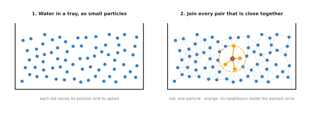
The red particle is joined only to the orange ones inside the dashed circle, so only those influence it.
Because particles move and their neighbours change, the graph is built again at every step. Which of those two kinds of join a model uses is the first thing to decide in the shortlist. GNS, in section 5.3, rebuilds the whole graph from the connection radius at every step, which is what water, sand and dough need. MeshGraphNets, in section 5.4, keeps the mesh's own threads, which is what cloth needs. VCD, in section 5.5, covers the case where nobody can hand you the mesh, because it learns which of the points the camera can see are joined.
The difference between those two ways of joining is worth spelling out, because it decides what the model can and cannot know.
When the graph is built from particles, a join means only "these two were close just now". The joins are thrown away and made again at every step, so a join appears the moment two particles come near each other and disappears when they move apart. That is right for water and sand, where the neighbours really do change. It also has one consequence that is easy to miss. The model cannot tell "this is the same piece of material" from "this is a different thing that happens to be touching". Two separate lumps of dough pressed together become one connected body, with no extra work from anybody, which is what you want for dough and wrong for a towel folded onto itself.
When the graph is built from a mesh, a join means "these two points are held together by the material itself". Those joins are given once and never change, however the cloth moves. So two points stay joined when the towel is bunched up, and two parts of the towel that are pressed against each other stay unjoined. The price is that something has to hand you the mesh, and a depth camera does not. A mesh model then adds a second, smaller set of distance-based joins on top of the mesh's own, for the places where the material touches the gripper or itself, and section 5.4 describes how MeshGraphNets keeps the two kinds apart.
One step: passing messages#
Each step has three parts, and they happen to every particle at the same time.
This step is the one Interaction Networks introduced in 2016, and section 5.1 keeps that paper in the shortlist because it is the clearest explanation of the step and nothing else. The models you would actually run are the later ones in the same list.
- Each neighbour sends a message. A small network looks at a pair of joined particles: their positions and their speeds. It gives back a short list of numbers, called a message. You can think of the message as "how much this neighbour pushes or pulls on me". Nobody tells the network what the message should be, because it learns whatever numbers help the prediction.
- The particle adds up its messages. It sums all the messages it received, and adds gravity.
- It moves a small step. A second small network turns the sum into a change of speed, and the program adds that to the particle's speed and moves the particle.
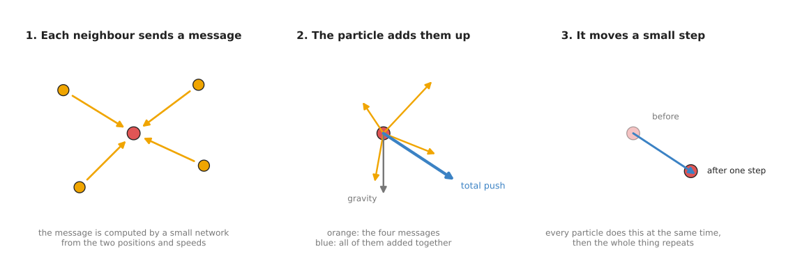
So every particle does this at once, and then the whole process repeats for the next step.
Two things about that step are worth saying plainly, because everything else on this page rests on them. The first is what a message actually is. It is a short list of numbers and nothing else. Calling it "a push or a pull" is a convenience for the reader, because nothing in the model labels those numbers, and if you printed them they would mean nothing to you. What makes them useful is only that the two small networks were trained together, so whatever the first network writes is what the second network has learned to read.
The second is why the messages are added up rather than combined in some cleverer way. A particle has however many neighbours it happens to have, and that count changes from particle to particle and from step to step. Adding is one of the few ways of combining a list whose length keeps changing, and it has the property the whole design depends on: the answer does not depend on the order the messages arrived in, and it does not depend on how many of them there were. That is why one trained model copes with a particle that has three neighbours and a particle that has thirty.
Parts 1 and 2 are usually repeated several times within one step before part 3. Each repeat lets information travel one more join across the graph, so after ten repeats a particle is influenced by particles up to ten joins away. This is how a pull on one corner of a towel reaches the far corner. The number of repeats is a setting, and NVIDIA's defaults for MeshGraphNets, which section 5.4 recommends, are 15 message-passing blocks of 128 numbers. DPI-Net, in section 5.2, is the step from a few objects joined to each other to a cloud of particles that an arm pushes around.
The same small networks are used for every particle and every pair, and this is the key idea of the whole design. The model learns one rule for "how neighbours affect each other", and it does not learn a separate rule for every particle. So a model trained on a small towel can often run on a bigger towel, which simply has more particles.
Many steps#
To predict a whole fold or a whole pour, the simulator runs many steps in a row, feeding each result back in. This is the rollout from the learned dynamics models page. So learned simulators often run hundreds of steps, because each step is short. Errors add up here too.
4. How it is trained#
The sections above described the model, and this section says where its examples come from. A learned simulator needs examples of the material moving, with the position of every particle at every step, and there are two places to get them.
The first place is a hand-written simulator that is very accurate but slow. Engineers already have careful simulators for cloth, fluids and sand, and these can take a long time to compute each step, but they give the exact position of every particle. So the learned simulator watches thousands of runs and learns to copy them: it predicts one step, is compared with the careful simulator's next step, and is corrected. This is where the published GNS and MeshGraphNets models in section 5.3 and section 5.4 come from.
The second place to get examples is the real world itself. The robot pokes, pinches or lifts the material while a depth camera records it, and this teaches the model the real material rather than a simulated one. However, it is harder, because a camera cannot say which dot in one frame is the same bit of material as which dot in the next frame. So the training compares the predicted shape with the real shape as a whole: for each predicted dot, how far is the nearest real dot? RoboCraft and RoboCook, in section 5.6, are the entries that learned this way, and that is the whole reason they are in the shortlist.
Because the data is cheap, training on simulated runs is common. Then a small amount of real data is often added, so that the model matches the real material.
5. Well-known models of this kind#
The models below are all real, published models, and this section is here so that
you can pick one. It has to be plain about one thing first. Of all the model
families in this book, this is the one where the distance between a published
demonstration and a program you can run is widest. Most of what follows is
research code, two entries need a graphics-card library compiled from source
before anything starts, and only one is installed with pip.
Read the table one row at a time. The left column names the model and says how
current it is. The right column holds the rest: what the model is best at, how
big it is, its licence, and when to pick it. Read what each row says about size
carefully. Almost nothing in this family publishes a parameter count or a memory
requirement, so you cannot work out what hardware you need by reading a paper,
and that absence is itself one of the findings of this section. A row says not stated where the number is not published, rather than giving a guess.
| Model | What decides it |
|---|---|
| 5.1 Interaction Networks, historical | It is best at explaining how all the others work. Its size is not stated, and no code was released. Pick it when you want to understand the idea rather than run it. |
| 5.2 DPI-Net, historical | It is best at rigid, soft and liquid objects together. Its size is not stated, and neither repository has a licence file. Pick it when you are reading a paper that compares itself with it. |
| 5.3 GNS, most used in 2026 | It is best at water, sand and dough-like material. Its size is not stated, and its datasets run from 2,000 to 14,000 particles. The code is Apache-2.0, and no licence is stated for the datasets. Pick it when your material has no fixed set of joins. |
| 5.4 MeshGraphNets, most used in 2026 | It is best at cloth and anything else with a mesh. No parameter count is stated, and NVIDIA's defaults are 15 message-passing blocks of 128 numbers. Both implementations are Apache-2.0. Pick it when you have a mesh and want maintained code. |
| 5.5 VCD, historical | It is best at smoothing a crumpled cloth from one camera. Its size is not stated, and the licence is MIT. Pick it when the joins must be guessed from what the camera sees. |
| 5.6 RoboCraft and RoboCook, worth betting on | They are best at real dough and plasticine on a real arm. Their size is not stated, and the licence is MIT. Pick them when your material is real and nobody has measured it. |
5.1 Interaction Networks#
This model is historical, and it is here because every other model on this page is a variation on it.
Size not stated, a laptop for the fifteen lines below, and no licence at all, because no code was released.
Peter Battaglia and others at DeepMind published Interaction Networks for Learning about Objects, Relations and Physics in 2016. It predicts how a few objects move by sending one message along each connection between a pair of them and then adding up the messages each object received, which is the step that section 3 described.
The one idea it is built on is that a physical scene can be written down twice over: once as a list of objects, and once as a list of the pairs that affect each other. The network then learns one rule for each list. One small network says what happens between a pair, and one small network says how an object moves given everything that happened to it. All the physics the model knows lives in those two networks, and there is nothing else in it.
What that changes inside the model, compared with every later entry here, is where the list of pairs comes from. In Interaction Networks it is written down by hand and stays the same for the whole prediction. There is no connection radius and no rebuilding. The graph that section 3 describes is given to this model rather than worked out by it, so two objects that were not listed as a pair cannot affect each other, no matter how close together they end up.
That buys you a model small enough to hold in your head, and a rule that does not care how many objects there are, because the same two networks are used for every pair and every object. What it costs is that somebody has to know the pairs in advance. Contact is exactly the case where nobody does, since a contact exists for a few steps and then stops existing. DPI-Net in 5.2 is the entry that fixes this, and the fix is the first thing it is named after.
On a robot arm the difference shows up as soon as the material can touch itself. A rope described as ten beads in a line is a scene it handles well, because the pairs are the links of the chain and they never change: you write the list once. Then the rope folds over and one bead presses down on another twenty beads away along the chain. Nothing in the hand-written list says those two beads interact, so the model predicts the rope passing through itself, and the prediction is useless from that step onward. That single failure is why the rest of this page rebuilds the list from distances instead.
You would not choose it over GNS in 5.3 for real work, because GNS is the same idea with the extra parts that keep it stable over hundreds of steps. The reason to read this paper first is that it has only two small networks and nothing else, so every later model then reads as a small change to something you already understand.
The one cost worth recording is that no code was released with the paper, and DeepMind's research repository lists its later graph simulators but not this one. You write it yourself, which is reasonable, because the whole model is about fifteen lines.
The library that makes those fifteen lines possible is PyTorch Geometric, which
adds graphs to PyTorch, and you install it with
pip install torch torch_geometric:
import torch
from torch_geometric.nn import MessagePassing, radius_graph


class ClothStep(MessagePassing):
    def __init__(self):
        super().__init__(aggr="add")            # each particle adds its messages up
        self.message_net = torch.nn.Sequential(
            torch.nn.Linear(12, 64), torch.nn.ReLU(), torch.nn.Linear(64, 32))
        self.update_net = torch.nn.Sequential(
            torch.nn.Linear(38, 64), torch.nn.ReLU(), torch.nn.Linear(64, 3))

    def message(self, x_i, x_j):                # x_i receives, x_j sends
        return self.message_net(torch.cat([x_i, x_j - x_i], dim=1))

    def forward(self, particles, edge_index):
        summed = self.propagate(edge_index, x=particles)
        return self.update_net(torch.cat([particles, summed], dim=1))


# 200 points spread over 20 cm of towel, each with 3 positions and 3 speeds
particles = torch.rand(200, 6) * 0.2
edge_index = radius_graph(particles[:, :3], r=0.03)   # joined if closer than 3 cm
change_in_speed = ClothStep()(particles, edge_index)
The library gave you two things.
radius_graph
rebuilds the graph from the current positions, and aggr="add" collects each
particle's messages. Notice that message is given the difference between the two
positions rather than the two positions themselves, so that the same rule works
anywhere on the table.
Everything else is yours to write. The two small networks start from random
numbers and know nothing until they are trained, as
section 4 describes, and you still have to turn a point
cloud into particles, add gravity and the gripper, repeat the message step
several times before anything moves, and run many steps in a row for a whole
fold.
5.2 DPI-Net#
This model is historical, and it is here because it is the step from predicting a few objects to predicting a cloud of particles that a robot arm pushes.
Size not stated, an NVIDIA card whose memory nobody states, and no licence file in either repository.
Yunzhu Li and others published Learning Particle Dynamics for Manipulating Rigid Bodies, Deformable Objects, and Fluids at the International Conference on Learning Representations in 2019. It handles rigid blocks, soft objects and water in one framework and uses the learned model to plan how to manipulate them.
The one idea it is built on is in the first word of its name, which stands for dynamic particle interaction networks. The list of pairs is made again from the particles' current positions at every step, so a pair starts interacting when it comes close and stops when it moves apart. The paper's reason for this is worth quoting, because it says what Interaction Networks got wrong: a fixed list of pairs assumes the forces between things change smoothly, and "many physical interactions involve discontinuous functions (e.g. contact)". A contact is not a smooth thing. It is either there or it is not.
Two more parts follow from that, and both are about distance. The first is that the message step is repeated several times inside one prediction step, which section 3 described, so that a push can travel several joins before anything moves. The second is a hierarchy, and it is the part that is unique to this entry. The particles of an object are sorted into groups, and each group gets an extra particle of its own, which the paper calls a root. Messages then travel in four stages: between ordinary particles, from ordinary particles up to their root, between the roots, and back down from the roots to the particles. A root is a shortcut, so one end of a long rigid block hears about the other end in a few hops rather than in as many hops as there are particles between them. For a rigid object the model goes further still: the signals on an object's particles are averaged into a single rotation and translation for the whole object, and every particle is then moved by that one transform.
What that buys is rigid, soft and liquid material in a single framework, and rigid objects that stay the shape they are, which a flat graph cannot promise. What it costs is that the grouping is yours to supply. You have to say which particles belong to which object and how they are grouped, and a wrong answer is visible: a block that is split into two groups the model treats as two independent rigid bodies will hinge in the middle. The rebuilt list also makes each step more expensive than Interaction Networks', because the neighbour search runs every time.
On a robot arm the case where this matters is an arm pushing into a stack of blocks. With Interaction Networks you would have to list every pair of blocks that might ever touch before the push starts, and the stack's whole point is that you do not know. DPI-Net finds the pairs as the stack collapses. Then, because each block has a root and a rigid transform, the blocks are still cubes a hundred steps later, where a model that predicts each particle on its own leaves you with blocks that have slowly sagged into pillows.
You would not choose it over GNS for new work, because GNS came later from the same research line and is the design other papers now compare themselves with. Its own authors replaced it as well, with VGPL-Dynamics-Prior, which they describe as adding noise to the particle positions during training for more stable long rollouts. That is the fix, and here you can see the setting that switches it on.
What it costs you is mostly the installation. The original repository needs PyFleX, a particle simulator that has to be compiled against CUDA, so an NVIDIA card is not optional. The successor can draw its predictions with VisPy instead, which is an ordinary Python package. The training data is two downloads from Dropbox, of 1.14 GB and 2.9 GB, fetched by hand.
The library is plain PyTorch, and the successor repository is the one to run, because it ships a trained model and a small amount of validation data:
git clone https://github.com/YunzhuLi/VGPL-Dynamics-Prior.git
cd VGPL-Dynamics-Prior
# Rolls the shipped model forward on the demo data for a falling pile of rigid blocks
bash scripts/dynamics/eval_RigidFall_dy.sh
What you get is a working particle predictor and two scenes, which are falling
rigid blocks and a rope with a mass on the end. What you supply is your material,
your camera, and a way of turning a point cloud into the format its loader
expects. The settings are passed on the command line inside those shell scripts:
--n_his 4 is how many earlier frames the model sees, --augment 0.05 is the
size of the training noise described above, and --vispy 1 turns on the drawing.
5.3 Graph Network-based Simulators (GNS)#
This model is most used in 2026 in the sense that matters when you read papers, because it is the design new particle simulators compare themselves with.
Size not stated, a graphics card whose memory nobody states, Apache-2.0 for the code and nothing stated for the datasets.
Alvaro Sanchez-Gonzalez, Jonathan Godwin, Tobias Pfaff, Rex Ying, Jure Leskovec and Peter Battaglia published Learning to Simulate Complex Physics with Graph Networks at the International Conference on Machine Learning in 2020. It learned water, sand and a sticky goo-like material from a careful hand-written simulator, with one design and one set of settings for all three.
The one idea it is built on is that the material should not be part of the design. In DPI-Net you tell the model how the particles are grouped and which object is rigid. In GNS you tell it nothing of the sort. Each particle simply carries a label saying what it is made of, and water, sand, goo and the walls of the container are four values of that one label. One set of small networks then learns how water affects water, how sand affects sand and how either affects a wall, all inside the same weights, and it learns that from the label rather than from a separate model per material.
Inside, that leaves a flat graph and three stages. The first stage builds the graph from the connection radius and turns each particle and each join into a list of numbers. A particle's numbers are its position, its last five speeds, and that material label. A join's numbers are the offset from one particle to the other and how far apart they are, which is what makes the rule work anywhere on the table rather than only where it was trained. The second stage is the message step of section 3, repeated a fixed number of times. The third stage reads the result off each particle as one acceleration, which is added to the particle's speed. Nothing here is grouped, nothing is rigid, and no root particles exist.
One further part is what makes GNS usable over hundreds of steps, and it is not
in the architecture at all. During training, random noise is added to the speeds
the model is given, so it is trained on slightly wrong inputs. The reason is the
rollout. In training the model is handed the simulator's exact state, but in a
rollout it is handed its own previous prediction, which is slightly wrong, and a
model that has only ever seen exact inputs does not know what to do with a wrong
one. The errors then grow until the water explodes. Noise during training makes
the two situations look alike. DPI-Net's successor repository added the same fix
afterwards, which is the --augment setting 5.2 points at.
What the flat graph buys you is that the material can change its shape and its connections completely and the model does not care. What it costs is twofold. Nothing enforces a rigid shape, so a solid object in a GNS scene holds together only as well as the network learned to hold it together. And the material label is a short fixed list, so a material that was not among the training values has no label to be given, and you retrain. There is also a practical catch in those five previous speeds: you cannot start a prediction from one camera frame, because the model wants a short run-up of frames before it will say anything.
On a robot arm the difference from MeshGraphNets shows up when two separate pieces of material become one. The arm presses two lumps of dough together. In GNS the joins are rebuilt from distance, so at the step where the lumps touch they are one connected body and the pressure travels through both, with nobody having edited anything. A mesh model cannot do that, because its joins were fixed before the run and no join exists between the two lumps. The same property is what makes GNS wrong for the towel in 5.4, where two layers touching must not become one piece of cloth.
You would choose it over MeshGraphNets in 5.4 when your material has no fixed set of joins. GNS takes a bag of particles and rebuilds the graph from distances at every step, which is what water, sand and dough need, because a grain of sand's neighbours change constantly. MeshGraphNets expects a mesh whose joins stay the same. Cloth has one and a pile of sand does not.
What it costs you is a dead software stack. The reference code pins
tensorflow>=1.15,<2, which is TensorFlow 1, and lists the retired sklearn
package name, so you build a Python environment nothing else you own will share.
The datasets are TFRecord files served from a Google Cloud Storage bucket, and
nothing states what you may do with them. The deeper cost is that the published
model learned from a hand-written simulator, so it knows a simulated material
rather than a real one.
The library is not a library. It is a folder called learning_to_simulate inside DeepMind's research repository, which you clone and read:
git clone https://github.com/google-deepmind/deepmind-research.git
cd deepmind-research
pip install -r learning_to_simulate/requirements.txt   # pins TensorFlow 1.15
# WaterRamps is water poured over fixed ramps
bash ./learning_to_simulate/download_dataset.sh WaterRamps /tmp/datasets
python -m learning_to_simulate.train \
    --data_path=/tmp/datasets/WaterRamps --model_path=/tmp/models/WaterRamps
The download gives you more than particle positions. Each dataset carries a
metadata.json file stating the sequence length, the number of dimensions, the
box the material sits in, the default connection radius and the statistics used
to normalise the numbers. Those settings decide whether the model is useful, so that file is the fastest way to see sensible values.
What you supply, in practice, is a different implementation. Because TensorFlow 1 is no longer reasonable to install, people either rewrite the GNS design in PyTorch using the step from 5.1, or take NVIDIA's version described next, which trains on these same datasets. Use the DeepMind folder as the specification and the datasets as training data.
5.4 MeshGraphNets#
This model is most used in 2026 and it is the one to start from, because it is
the only model on this page with a maintained implementation inside a library you
install with pip.
Size not stated, a graphics card, Apache-2.0 for both implementations.
Tobias Pfaff, Meire Fortunato, Alvaro Sanchez-Gonzalez and Peter Battaglia published Learning Mesh-Based Simulation with Graph Networks at the International Conference on Learning Representations in 2021. It keeps the mesh's own edges as joins, so a pull on one corner of a flag travels along the threads of the cloth rather than through whatever happens to be nearby in space.
The one idea it is built on is that "connected by the material" and "close in space" are two different relationships, and a model that has only one kind of join is forced to confuse them. GNS has one kind, built from distance. A towel folded in half has two layers almost touching, and in GNS a pair of facing points across that fold is joined exactly like a pair of neighbours along the same thread. MeshGraphNets refuses to merge the two.
So inside, each particle has two sets of joins instead of one, and each set has its own small network. The mesh joins come from the mesh and never change; the numbers on a mesh join are measured in the cloth's own flat, unstretched coordinates, so the join says how far apart the two points are along the fabric, whatever the towel is doing in the air. The second set is called world joins in the paper, and they are added at every step between points that are closer than a small distance in space but not joined on the mesh. The paper is direct about the division of labour: mesh joins let the network work out the material's internal behaviour, and world joins "can estimate external dynamics, not captured by the mesh-space interactions, such as contact and collision". The three stages are the same as GNS's, and the number of repeats of the message step is the setting NVIDIA's default of fifteen blocks refers to.
One more part has no equivalent in GNS. The model can also predict how fine the mesh should be at each point, which the paper calls a sizing field, and an ordinary remeshing program then splits or merges triangles while the prediction runs. So the mesh is not frozen at the resolution it was trained on: it can get finer where the cloth is bending sharply. This is the part that keeps a mesh-based model from being stuck with whatever shape its training data had.
What two kinds of join buy you is that cloth touching cloth stays two pieces of cloth. What they cost is the mesh itself, and this is where the whole entry becomes awkward on a real arm. A mesh is not just a set of joins. The flat coordinates mean you have to know which point of the fabric is which, and a depth camera gives you a heap of unlabelled dots with no idea which one used to be the top left corner. So on a robot arm, this is the model to use when the cloth is held in a known way or when a separate step has fitted a mesh to it, and 5.5 is the entry for when nobody can do that. The concrete case is an arm holding a towel by two corners so that it hangs in a U, with the two halves facing each other a centimetre apart: GNS joins those facing points with the same network that handles threads, and the towel it predicts sticks to itself, whereas MeshGraphNets hands them to the network that learned contact.
You would choose it over GNS whenever your material has a mesh, and cloth is the case that matters for a robot arm. There is also a reason that has nothing to do with physics. NVIDIA maintains a PyTorch implementation inside PhysicsNeMo, with current dependencies, while every other entry here is a research repository you keep alive yourself.
What it costs you, beyond the mesh, is which implementation you take. DeepMind's
own release is in GNS's state: it asks for tensorflow-gpu>=1.15,<2 and Python
3.6, and ships a complete pipeline for only two scenes, cylinder_flow and
flag_simple. NVIDIA's version is current but assumes an NVIDIA card in several
places. Its particle example sets the test device to cuda, and its graph
dependencies install as an extra, with
pip install "nvidia-physicsnemo[cu13,gnns]".
The model is one class. This builds the network for one step of a towel and runs it once:
import torch
from torch_geometric.data import Data
from torch_geometric.nn import radius_graph
from physicsnemo.models.meshgraphnet import MeshGraphNet

# 200 points over 20 cm of towel, each with 3 positions and 3 speeds
particles = torch.rand(200, 6) * 0.2
edge_index = radius_graph(particles[:, :3], r=0.03)    # joined if closer than 3 cm
graph = Data(edge_index=edge_index, num_nodes=particles.shape[0])

# One feature per join: the offset from the sending particle to the receiving one
sender, receiver = edge_index
edge_features = particles[sender, :3] - particles[receiver, :3]

# The defaults are 15 message-passing blocks of 128 numbers, summed at each particle
model = MeshGraphNet(input_dim_nodes=6, input_dim_edges=3, output_dim=3)
change_in_speed = model(particles, edge_features, graph)   # one row per particle
Compare this with the code in 5.1 to see what the
library did. The fifteen repeats of the message step, the small networks that
encode the particles and the joins first, and the network that turns the result
back into three numbers are all inside MeshGraphNet, and the three sizes you
passed are the only shapes you had to get right.
What you still supply is the mesh and the training, because this network is untrained and the numbers above are meaningless. NVIDIA ships a worked example for this family at examples/cfd/lagrangian_mgn, which trains it on the GNS datasets, and its configuration file holds real values: five frames of movement history per particle, six kinds of particle, and twenty training passes over the data.
5.5 VCD#
This model is historical, and it is here because its one idea is reused by every cloth system that came after it: model only the part of the cloth the camera can see.
Size not stated, an NVIDIA card, MIT.
Xingyu Lin, Yufei Wang, Zixuan Huang and David Held published Learning Visible Connectivity Dynamics for Cloth Smoothing at the Conference on Robot Learning in 2021. It trains two networks. The first guesses which visible points are joined, and the second predicts how the joined points move. Then it plans pick-and-place moves that smooth a crumpled cloth.
The one idea it is built on is that if the mesh is what MeshGraphNets needs and no camera can supply it, then the mesh is something to predict rather than something to be given. VCD treats "are these two points joined by fabric?" as one more question for a neural network to answer.
Inside, that puts a whole extra network in front of the one this page has been describing. The point cloud is first thinned onto a grid so the points are spread out evenly. Then every pair of points closer than a chosen distance becomes a candidate, exactly as in GNS, but a candidate is not yet a join. A graph network looks at each candidate and answers yes or no: is this pair also joined on the real cloth? That classifier was trained inside a simulator, where the answer was known, because the simulator can say whether the two particles behind those two points share a spring. Only the candidates it says yes to are passed on. The second network is then the ordinary dynamics network of section 3, running on the graph the first one produced together with the collision joins, and predicting an acceleration for each point.
The way it acts is also different from everything else here, and it is worth knowing before you borrow the idea. VCD does not roll a long prediction forward. It considers one pick-and-place at a time: it samples where to pick and where to place, predicts the shape of the cloth after that single move, and keeps the move whose predicted shape covers the most table. Then the camera looks again. So the planning is greedy, one move deep, and the model is never asked to be right a hundred steps later, which is part of why the approach works at all from input this poor.
What the guessed mesh buys you is that one overhead camera is enough, and that is a large thing. What it costs is that the joins are now a prediction, and a wrong prediction is wrong physics with no warning attached. Worse, the part of the cloth the camera cannot see is not modelled at all, so a fold tucked under the top layer does not exist for the model, and the model cannot know it will unroll when the corner is pulled. The classifier also learned what cloth joins look like from one simulator's cloth. On a robot arm this is the entry for a towel dumped in a heap under a fixed overhead camera, where MeshGraphNets cannot even start, because there is no mesh and no way to say which dot was the top left corner. Ask VCD instead to predict a two-handed fold several steps ahead and it has nothing to offer, because the layer doing the work is the hidden one.
You would choose this idea over MeshGraphNets when nobody can hand you the mesh. MeshGraphNets needs the joins, including the ones under a fold, and a depth camera cannot see under a fold. VCD builds its graph from the visible points and learns the joins from training examples, which is the situation a real arm with one overhead camera is always in.
What it costs you is the installation, and this is the step at which people stop. VCD is a cut-down copy of a larger research framework and needs SoftGym, which needs PyFleX compiled from source against CUDA. The authors do publish trained weights, so you can see it work without training it.
The library is plain PyTorch, and the published planner runs from the command line. The two paths are the two networks:
# vsbl is short for "visible": both networks work on visible points only
python VCD/main_plan.py --edge_model_path ./data/vcd_edge/vsbl_edge_120.pth \
                        --partial_dyn_path ./data/vcd_dyn/vsbl_dyn_120.pth
What you get is the whole published pipeline: the join-guessing network, the movement network, the planner and the cloth scenes. What you supply is a real camera and a real cloth, because all of the above runs inside the simulator the paper used, and the authors did not publish the part that replaces the simulator's point cloud with a camera's.
5.6 RoboCraft and RoboCook#
These models are worth betting on, because they are the only entries here that learned a real material from a real arm rather than from a hand-written simulator, and that is where the argument for this family leads. A model trained on a careful simulator has not avoided that problem, because it inherited whatever numbers the simulator was given. A model trained on recordings of real dough has.
Size not stated, an NVIDIA card on Ubuntu 18.04 or 20.04, MIT.
Haochen Shi and others published RoboCraft in 2022 and RoboCook in 2023. Both learn a particle model of elastic and plastic material from depth-camera recordings of a real arm squeezing it. The RoboCraft paper states the figure that makes the case: ten minutes of real interaction data was enough to learn a model that could shape the material into target shapes it had not seen before. RoboCook uses several tools in sequence and also learns to choose the tool, and its published demonstration makes dumplings.
The one idea these two are built on is that the particles should come from the cameras rather than from a simulator. Everything else on this page starts from a state somebody already has: a simulator's particles, or a mesh. These start from four calibrated depth cameras pointed at a lump of real dough.
What that changes is the front of the pipeline, not the graph network. RoboCook merges the four point clouds, cuts the dough out of the scene by its colour, builds a closed surface around the remaining points, and then draws particles both inside that surface and spread evenly over it. The important consequence is that a particle is a fresh sample every time, not a piece of dough that keeps its identity from frame to frame. So the training cannot compare particle number seven with particle number seven, which is why it uses the whole-shape distances section 4 described, and the paper names two of them: Chamfer distance, which asks how far each predicted point is from the nearest real point, and Earth Mover's distance, which asks how much work it would take to move the predicted shape onto the real one.
RoboCook then adds a part that no other entry here has, which is choosing the tool. A separate point-cloud network reads the dough's shape now together with the shape you want, and gives a probability for each of fifteen tools. The three most likely tools are rolled forward through their own dynamics models, and the tool whose predicted result lands closest to the target is the one that gets used. Notice "their own": the dynamics model is per tool, which is why the repository ships one dynamics dataset per tool rather than one for the task.
What this buys you is a model of the material in front of you, including the stiffness and the spring-back that nobody wrote down. What it costs is that nothing transfers. Add a tool and you record real data again, train again, and extend the classifier, where in GNS a new material is at worst a retraining on data somebody else generated for free. On a robot arm the difference is simple and sharp: an arm pressing a roller into real dough, where GNS trained on simulated goo gets how far the dough spreads and how much it springs back wrong, because it learned a simulator's goo and nobody measured this dough. RoboCook's model watched this dough. Ask it instead about a tool it has never held, and it has no answer at all, while GNS at least has a material label to put it under.
You would choose this over GNS when your material is real and unmeasured. GNS learned from a simulator, so it knows a simulated material well. RoboCook learned from a real gripper pressing real dough, and it is the only published recipe that matches the situation of somebody with a real arm, a real soft material and no measurements of it.
What it costs you is a different computer. The repository states its prerequisites as Ubuntu 18.04 or 20.04, so a Mac will not do. The recorded data is on Google Drive and downloaded by hand, and it arrives split per tool: seven dynamics datasets, one per tool, and fifteen tools for the part that chooses between them.
The library is plain PyTorch, driven by shell scripts:
git clone https://github.com/hshi74/robocook.git
cd robocook
git submodule update --init --recursive
conda env create -f robocook.yml && conda activate robocook
# Trains the particle model on the recorded real dough for one tool
bash scripts/dynamics/run_train.sh
What you get is the recorded real material, which is the expensive part you
cannot reproduce quickly, together with the model, the tool classifier and the
planner. What you supply is your own tool, your own camera and the calibration
between them. Read the top of scripts/dynamics/run_train.sh first, because every
setting is there and each one names the section of the paper it comes from. The
one to look at is neighbor_radius=0.01, which its own comment describes as the
radius used to connect edges in the graph, so for real dough the published value
is one centimetre.
5.7 How to choose#
Start with MeshGraphNets through NVIDIA's PhysicsNeMo, because it is the only model here that installs as a package and the only one somebody else is maintaining.
Four things change that choice. If your material has no mesh, because it is water, sand or dough, follow the GNS design instead: download the GNS datasets for their metadata and their recorded positions, but build the model with PhysicsNeMo's particle example rather than with DeepMind's TensorFlow 1 code. If your cloth is crumpled and you have one overhead camera, take VCD's idea of guessing the joins between visible points, which you will probably rewrite rather than install. If your material is real, nobody has measured it, and you have a Linux machine with an NVIDIA card, start from RoboCook, because it is the only entry whose training data came from a real arm. If you only need to understand the family, read the Interaction Networks paper and the fifteen lines in 5.1, and stop there.
One more case changes the answer completely, and it is the most common one. If
your objects are rigid, or if the few numbers describing your material can be
measured, do not use any of these models.
MuJoCo 3.14.0, released on 22 September
2026, added an experimental contact mode called ipc that guarantees
penetration-free contact on deformable meshes, which is the failure that made
hand-written cloth simulation untrustworthy. Book 3's
MuJoCo section
also records the limits of that mode, and they are severe: those contacts are
frictionless, which rules out most grasping, and exact replay of a run is not
supported. So a written simulator is now the better choice for more cloth problems
than it was a year ago, and it is still the wrong choice for a towel you have to
grip.
6. Where this is going#
This section looks forward rather than back, and it was written on 4 October 2026. Book 3 sorts forward-looking statements into four kinds, in four kinds of claim: a demonstration is a recording of something working once under conditions the publisher chose, a product announcement says a thing can be bought or downloaded, a research result is a measured number on a stated task, and a projection is a statement about a date that has not arrived. This section names the kind every time, and says so where the judgement is mine rather than somebody's published statement.
The shape of the change in this family was never the architecture. Interaction Networks already had the two small networks that every entry in section 5 still uses. What moved was where the list of pairs comes from, which went from a hand-written list to a list rebuilt from distance at every step, and then where the training data comes from, which went from another simulator's output to a real arm's recordings. The second move is the one still in progress, and it is the one the rest of this section is about.
No robot cell in production runs a learned simulator, and the clearest evidence is where the maintained code lives. NVIDIA's PhysicsNeMo, which section 5.7 sends you to, reached version 2.2.2 on 11 September 2026 and is the only maintained home of MeshGraphNets. Its examples folder has areas for weather, computational fluid dynamics, structural mechanics, molecular dynamics, reservoir simulation, nuclear engineering, additive manufacturing and healthcare. It has no area for robotics. That is checkable today, and it says which industry pays for this family.
The industries that pay buy it as a product. Ansys sells SimAI, whose own page describes training a model from a customer's existing simulation results with no coding, and whose 2026 R1 release splits it into a desktop tier called SimAI Pro and a cloud tier called SimAI Premium. Siemens sells Simcenter PhysicsAI, which predicts fields directly on a mesh or a computer-aided design model and is embedded inside Simcenter Hypermesh and the design manager of Simcenter STAR-CCM+. Both are product announcements, the strongest kind of claim here, and both vendors are careful in the same way. The Siemens page's own answer to whether it can replace traditional solvers says that it complements them, and that critical designs should still be validated with a conventional solver. The same page relays a customer claim from Kinetic Vision of predictions up to 4,000 times faster at up to 97.5% accuracy, with no protocol attached, so read that as a claim rather than a measurement. Note what these products predict: the answer for a new shape, not a long rollout of changing contact, which is a different job from the one a robot arm needs done.
The one field where a learned simulator took over daily operational work is weather forecasting, and the most instructive event there is the one that went against it. The European Centre for Medium-Range Weather Forecasts has run its own machine-learning forecast system operationally since February 2025. On 11 May 2026 it published Farewell to the external AI models, which says it is stopping the real-time operation of four externally developed models: Google DeepMind's GraphCast, Huawei's Pangu-Weather, Microsoft's Aurora and NVIDIA's FourCastNet. The reason is a research result with a stated protocol: when its hand-written forecasting system was upgraded to a new cycle, the learned models that had been fine-tuned against the old one got worse, measured over two months of forecasts against the new cycle's own analysis. That is the moving-target problem in one experiment. A model trained on a written simulator's output inherits the version it learned from, and the written simulator keeps shipping.
The written simulators are where most of the current engineering effort actually
is, and that matters to anyone choosing between them and a learned model.
MuJoCo shipped eleven releases between February and September 2026, dated in
its changelog, and
three of them attack exactly the problems this page's models were built for.
Version 3.5.0 added a system identification toolbox, which fits masses,
frictions and motor gains to measurements from your own machine, and added
arbitrary delays
for actuators and sensors. Version 3.13.0, on 8 September 2026, added a
discrete integrator that keeps stiff springs stable at large timesteps.
Version 3.14.0, on 22 September 2026, added the experimental ipc contact mode
that section 5.7 already describes. Newton reached 1.6.0 on
10 September 2026, installs with pip install "newton[examples]", and its
README lists cable examples, cloth
examples including
a cloth held by a Franka arm,
material-point-method examples for granular material, water, snow and viscous
material, and differentiable examples including differentiable cloth.
Genesis World runs
multi-physics on an Apple Silicon Mac's own graphics processor. Every one of
those is a product announcement, checkable today, and together they answer
several of the cases this page recommends a learned model for.
The research front on the learned side has moved accordingly, and the move is away from replacing the simulator. AdaptiGraph learns a graph dynamics model that carries an estimate of the material's properties and updates that estimate while the arm pushes. PhysTwin fits a spring-mass model, a shape model and a set of Gaussian splats to a few videos of a real rope, cloth or stuffed animal, which means the learned part is the parameters and the state rather than the physics. Particle-Grid Neural Dynamics learns a hybrid of particles and a spatial grid from colour-and-depth video. All three are research results with published papers, and PhysTwin's code is on GitHub. Read them together and the direction is clear: the valuable output is a description of the material in front of you, which a solver can then use.
The second live front is getting the particles in the first place. A particle model cannot run without particle positions, and a camera sees one side of a crumpled towel. Book 3's section on real-to-sim reconstruction records that rebuilding a scene from a phone scan became a recurring published result through 2026, mostly using Gaussian splatting, and that most of that work is paper only rather than downloadable. Our scene reconstruction page covers the methods. Until that half is solved, a learned simulator on a real arm is a research project.
Three things remain unsolved, and the first is embarrassing rather than hard.
Nobody in this family publishes a parameter count, a memory requirement or a
shared benchmark. Section 5 says not stated in six rows for that reason. The consequence is that you cannot compare
two learned simulators, you cannot tell what hardware you need from a paper, and
a claim of improvement cannot be checked by anybody who did not write it. Ten
years of papers in this family have not fixed this, and no project has announced
that it will.
The second is that a learned simulator cannot promise anything. MuJoCo's ipc
mode makes non-penetration a guarantee by checking every step, and the price of
that guarantee is written in the changelog: the contacts are frictionless and
exact replay is not supported. A learned model offers no such trade, because
nothing in it can be checked. Long rollouts in this family are still kept
stable by adding noise to the inputs during training, which
section 5.3 describes, and that is a
patch that works rather than a bound on the error.
The third is that nobody has measured the materials. Book 2 explains that friction and softness numbers in a simulator are plausible rather than measured, and a learned simulator does not escape it. The published GNS and MeshGraphNets models learned from a hand-written simulator's guesses, and AdaptiGraph and PhysTwin estimate the numbers from video with nothing independent to check them against. I could not find a published measurement of a real dough's or a real towel's properties that a second group reproduced.
What follows is what I expect, and it is my judgement rather than anybody's commitment. I expect learned models in this family to be adopted as corrections on top of a written simulator rather than as replacements for one. The reason is the amount of data each job needs. Learning the whole physics of dough from scratch takes a dataset nobody on a robot project has; learning the difference between what MuJoCo predicts and what the real towel did takes far less, because the written simulator already supplies the part that is right. MuJoCo 3.5.0's system identification toolbox makes the written half fit your machine before the learned half is asked for anything, which is the step that was missing when GNS was published.
I expect the product that actually gets bought in robotics to be material identification rather than simulation. What a robot engineer lacks is not a solver; MuJoCo and Newton are free. What they lack is the stiffness and friction of the specific thing on their bench. AdaptiGraph and PhysTwin both attack that, and both hand their answer to a solver afterwards, which tells you where the value sits. This is a projection, and the thing that would confirm it is a released tool that takes a video of your material and returns parameters for a written simulator.
I expect mesh-based learned models to stay alive and particle-based ones to narrow to granular and liquid work. The reason is maintenance rather than quality. MeshGraphNets lives in PhysicsNeMo, which has releases, continuous integration and a company behind it. The reference code for GNS pins TensorFlow 1, as section 5.3 records, and nobody has announced a replacement. Adoption follows maintained packaging more reliably than it follows published accuracy.
I also expect the weather result to repeat in engineering, and this is the part worth carrying into how you read any paper in this family. A learned model trained on a written simulator's output has a shelf life set by the written simulator's release cycle. MuJoCo released eleven versions between February and September 2026 and changed the meaning of two contact parameters in one of them. A benchmark number produced against version 3.5.0 is not a number about version 3.14.0, and nothing in this family currently reports which version its training data came from.
The thing I do not expect, and I say so because the gap is the point of this page, is a learned simulator you can install and point at your own towel. No organisation has announced one. The distance between a published demonstration and a runnable program is wider in this family than anywhere else in this book, and nothing published in 2026 narrowed it. If that changes, it will show up as a package on the Python Package Index with a trained model and a licence file, and that is the thing to watch for rather than the next paper.
7. Where to read next#
- The next page covers latent world models, which predict a short code instead of particles or pictures.
- Point cloud models explain the 3D dots that a learned simulator starts from.
- Scene reconstruction covers building a whole 3D scene from pictures.
- Touch sensing models cover the sense that tells a gripper how soft a material is when it holds it.
- For the hand-written simulators that learned simulators are compared with, read Book 3's simulation and evaluation.