This page explains the simplest kind of world model, which is a learned dynamics model. It answers four questions: what such a model predicts, how a robot arm uses the prediction to choose what to do, how the model is trained, and when it is the right tool.
It is written for a reader who has already read the world models overview and the first chapter of this book, What models are. Because those pages explain what a model is, you should already know that a model takes a list of numbers in and gives a list of numbers back, and that it learns from examples. Beyond that starting point, no other machine learning is needed here.
Before this page, it helps to have read sampling-based optimisation and model predictive control, which explains the cross-entropy method and model predictive control that section 3 uses to plan, and system identification, which measures the numbers a physics model needs. Section 5 compares a learned model with that.
Contents#
- What it is
- What goes in and what comes out
- How it works inside
- How it is trained
- Learning only the part physics gets wrong: residual models
- Well-known models of this kind · 6.1 An ensemble of small networks, the PETS way · 6.2 A physics formula plus a learned correction · 6.3 TD-MPC2 · 6.4 MBPO, the model as extra practice · 6.5 PILCO, a Gaussian process model · 6.6 How to choose
- Where this is going
- Where to read next
1. What it is#
A learned dynamics model predicts the next state of the arm and the objects from the current state and an action.
Two words in that sentence need explaining, and the first of them is state, which is a short list of numbers that describes the scene right now. For example, for a cube on a table the state could be three numbers: where the cube is from left to right, where it is from front to back, and how far it is turned. The second word is dynamics, which means "how things move over time". So a dynamics model is a model of how the state changes over time.
Here is an everyday example of the same idea, using a shopping trolley in a car park. You know where the trolley is now, and you know how hard you push it. So from those two things you can guess where it will be one second later, and if you push it often enough, your guesses get good. Then you learn, without any formula, that a full trolley moves less than an empty one and that it drifts to one side. A learned dynamics model makes the same kind of guess, and it gets good at it in the same way, by seeing many pushes and where they ended up.
The word "learned" separates this model from the dynamics written in a physics textbook. A textbook formula for a sliding cube needs its weight and the friction between the cube and the table. A learned model needs neither of those numbers, because it only needs examples of the cube being pushed.
2. What goes in and what comes out#
Now that those two words are explained, here are the numbers themselves. A learned dynamics model takes two lists of numbers in and gives one list back.
- The state now. For example, the cube is at x = 0.30 m and y = 0.20 m, and it is turned 0°.
- The action. For example, the gripper pushes 0.10 m along x.
- The output: the predicted state after the action. For example, the cube will be at x = 0.38 m and y = 0.21 m, turned 15°.
The picture below shows this exchange of numbers. In this example four numbers go in, three for the cube and one for the push, and three numbers come out.
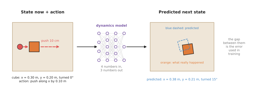
The dashed outline is the prediction, the solid cube is what really happened, and training tries to make the gap between them smaller.
Notice that the cube moved less than the push itself. The gripper travelled a full 10 cm, but the cube moved only about 8 cm and turned, because it slid and caught on one corner. A textbook formula would need the friction between the cube and the table to predict that. Instead, the learned model picks that friction up from the examples.
However, on a real arm the state usually has many more numbers than three. It holds the angle and speed of each joint, the position of each object, and sometimes how fast each object is moving. So a six-joint arm and one object can easily make a state of 20 numbers. The action is usually a small change in the gripper's position, or a target angle for each joint.
3. How it works inside#
One step#
The model itself is a small neural network of the kind described in inside a neural network. The state numbers and the action numbers are placed side by side in one list, and that list goes in at one end of the network. Then the predicted state comes out at the other end.
Many dynamics models predict the change in the state, not the new state itself. They output "the cube moves 8 cm along x and turns 15°", and the program adds that to the old state. This is easier for the network to learn, because the change is small and it looks similar wherever the cube is on the table.
The shortlist in section 6 recommends three other shapes for this one step, and they differ only in what the model is made of. Section 6.2 keeps a physics formula and learns only a small correction for what that formula gets wrong, and section 5 explains that shape in full. Section 6.5 uses a Gaussian process in place of the network, which means it fits a smooth curve through the recorded points rather than adjusting the weights of a network. TD-MPC2, in section 6.3, does not predict the state numbers at all. It predicts a short code of the state instead, which is what latent world models are about.
The rest of this section is written about the network, because that is the common case. The rolling forward and the planning it describes apply to all four shapes, though, because all four answer the same question about one step.
Many steps in a row#
One step is usually a short time, such as a tenth of a second. So to see further ahead, you have to use the model again and again. You feed its prediction back in as the next "state now", add the next action, and get the step after that. This is called rolling the model forward, and the list of predicted states is called a rollout.
Every step starts from the last prediction, not from the truth. So if step one is slightly wrong, step two starts from a wrong place and adds its own error, and the errors add up over the rollout. This is called compounding error, and it is the main weakness of every world model in this chapter.
Because the errors add up, you need a way to see how far a rollout can be trusted, and the usual way is to train several copies of the model. Each copy starts from different random numbers, so each one learns slightly differently. This group of copies is called an ensemble, and it is read in a simple way. Where the copies agree, the prediction is probably right, and where they disagree, the model has not seen enough examples of that situation. An ensemble of small networks is the first entry in the shortlist, and section 6.1 recommends it. A Gaussian process reports the same thing without any copies, because it states its own spread at every point.
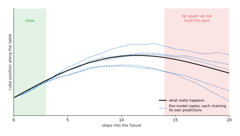
In this drawing of the idea, not a measured result, the copies start together and spread apart further into the future.
Planning with it#
Rolling the model forward is only useful if something then chooses the actions. That is what planning does, because planning means choosing actions by asking the model "what if?". A planner makes up many sequences of actions, rolls each one forward through the model, scores where each one ends up, and keeps the best. A method called the cross-entropy method, or CEM, repeats this a few times and narrows the search towards the best sequences. The arm then does only the first action, measures the real state again and plans again from there, and this loop is called model predictive control, or MPC. Because the plan is thrown away after one step, a wrong prediction five steps ahead does little harm. Book 6's sampling-based optimisation and MPC page teaches these methods step by step, with real numbers.
However, two things change when the model is learned. First, the planner searches for whatever the model says works best, so it is drawn to the places where the model is wrong in a hopeful direction. Second, the model is only trustworthy near its training records. This is why the ensemble matters: the planner uses the copies' average as the prediction, and it prefers sequences on which the copies agree. That same page has a worked example of a learned ensemble inside MPC that shows how much this helps.
Planning this way is what both section 6.1 and section 6.3 do. A dynamics model does not have to be planned with, though. MBPO, in section 6.4, rolls the model forward only while a policy is being trained, so that the policy gets extra practice, and then the model is put aside before the robot runs. The rest of this page describes planning, because that is the use which needs the model while the arm is moving.
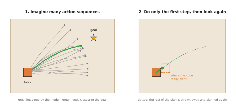
The planner tries many sequences inside the model, but the arm moves only one small step before it plans again.
4. How it is trained#
Planning only works once the model has been trained, so this section says where that training comes from. A dynamics model learns from records of the arm acting, and each record has three parts: the state before, the action, and the state after. The state is measured by the arm's joint sensors and, for objects, by a camera and a seeing model or by markers stuck on the objects.
The records come from three places, and the list below describes each one.
- Random play. The arm makes random pushes and small moves, and the system records what happens. This is simple, and it covers many situations.
- Demonstrations. A person guides the arm through the task, as described in where the data comes from.
- The robot's own attempts. Once the model is roughly right, the robot plans with it and tries the task. Each attempt gives new records, especially in the places where the model was wrong. The model is retrained, and the cycle repeats.
Once the records exist, training works as described in how a model learns. The network predicts the state after, the program measures the gap to the recorded state after, and it adjusts the network to make that gap smaller.
How much data is needed depends on the task itself. A dynamics model for one simple task, such as pushing one cube, is small, so it can often learn from tens of thousands of steps. For example, if the arm records 10 steps a second, then 10,000 steps is under 17 minutes of recording. A model that must cover many objects and many tasks needs far more than that.
5. Learning only the part physics gets wrong: residual models#
So far the network on this page has learned everything about how the cube moves, starting from nothing. However, there is a cheaper way when a physics formula already gets the answer roughly right. You keep the formula, and the network learns only the difference between the formula and what really happens. That difference is called the residual, which means "what is left over", and a model built this way is called a residual model. Some people call the method residual physics.
Here is an everyday example of the same split. A satnav, which is the device in a car that works out how long a journey will take, says the drive to work takes 20 minutes. However, you have driven it many times, and you know it always takes about 5 minutes longer on a Monday morning. You do not throw away the satnav and learn the whole road map yourself. Instead, you keep the satnav's answer and add your own small correction. In that example the satnav is the formula, and your 5 minutes is the residual.
How it works#
So the prediction is made in two parts, which are then added together.
- The physics part. A formula, or a physics simulator, predicts the next state from the current state and the action. It uses values from a table or a datasheet, such as the friction between wood and a table top.
- The learned part. A small network is given the same state and action, and predicts how wrong the physics part will be.
- The prediction is the physics answer plus the correction.
Training is the same as in section 4, with one change. For each record, the program first works out the physics answer. Then the network's target is the recorded answer minus the physics answer, not the recorded answer itself.
A worked example: how far a pushed block slides#
Here is a small example that the script for this page computes for real. The gripper pushes a wooden block along the table and then lets go, and the question is how far the block slides after that.
The physics formula for a sliding block says it stops after a distance of v² / (2 μ g). Here v is the speed when the gripper lets go, g is 9.81 m/s², the pull of gravity, and μ is the friction coefficient, which is a number that says how strongly the two surfaces resist sliding on each other. A table of materials gives μ = 0.30 for wood on wood.
The "real" block in the script is made to be a little different from those table numbers, as real blocks are. Its friction is higher than the table says, and it also rises with speed. The recorded distances have up to about 2 mm of measuring error as well. The learned part is a small model made of 8 smooth bumps, fitted by least squares . It stands in for a small network, because it behaves the same way for this purpose.
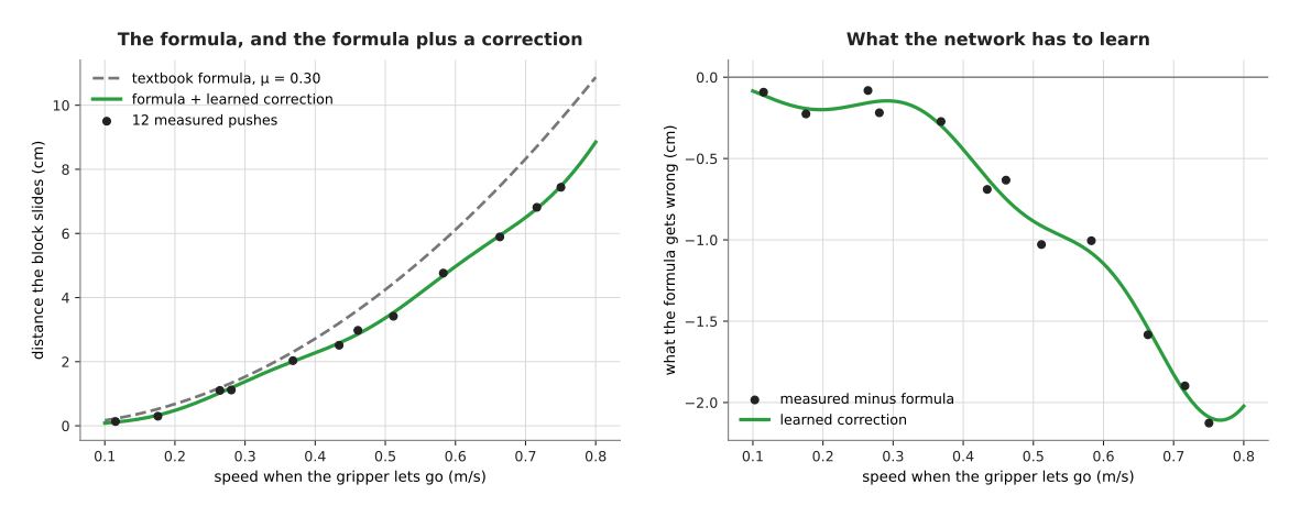
On the left, the dashed line is the formula, and it predicts too far at every speed. For example, at 0.5 m/s it says 4.25 cm, but the block slides 3.44 cm. On the right are the 12 measured pushes minus the formula, and this is all the network has to learn: a smooth curve from about 0 to about −2 cm. After fitting it to those 12 pushes, the formula plus the correction predicts 3.36 cm at 0.5 m/s. At 0.7 m/s the formula says 8.32 cm, the block slides 6.47 cm, and the formula plus the correction says 6.50 cm.
Why it needs less data#
The correction is easier to learn than the whole slide, and the next picture shows how much easier. It trains the same small model in two ways: in one the model learns the whole slide from nothing, and in the other it learns only the correction to the formula. Each point is the typical error over 200 repeats with different random pushes.
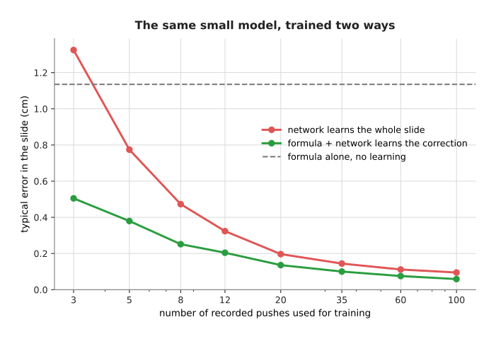
With 3 pushes, the model that learns the whole slide is wrong by 1.33 cm, which is worse than the formula alone at 1.14 cm. The residual model is wrong by only 0.50 cm. With 12 pushes the two are at 0.32 cm and 0.20 cm, and with 100 pushes both are good, at 0.09 cm and 0.06 cm.
The reason is simple, because the formula already knows the shape of the answer: faster pushes slide much further, and a push at zero speed slides nowhere. The model that learns everything has to discover that shape from the data. Instead, the residual model only has to learn a small, smooth correction, and a small, smooth correction takes few examples to learn.
Why it fails more gracefully#
The last picture asks both models about pushes that are harder than any they were trained on, because that is where a model usually breaks. Both were trained on 20 pushes at speeds between 0.1 and 0.45 m/s.
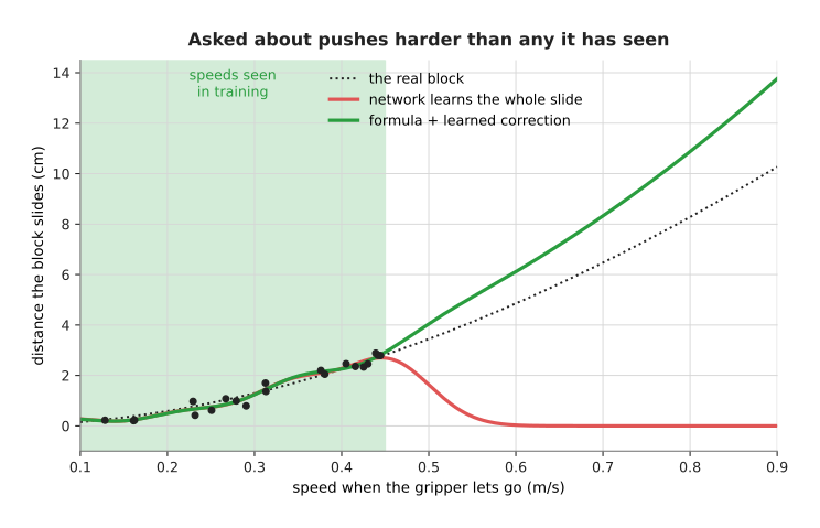
Inside the shaded band, both models are close to the real block. Outside it, however, the model that learned everything falls to almost zero. At 0.6 m/s it predicts 0.03 cm, when the block really slides 4.85 cm. That is not a small error, because it is a nonsense answer. The residual model instead falls back to the formula, and it predicts 6.11 cm. This is too far, but it is the right kind of answer, and it is exactly as wrong as the formula alone.
Be careful with that result, because it depends on the kind of model used. The bump model used here gives a correction of zero far from its data, so the residual model falls back to the formula by itself. However, a real network does not always do that. Some networks carry on in a straight line outside their data, so the correction can grow large. This is why people keep the correction small on purpose. They add a penalty on its size during training, cap it at a fixed limit, or use an ensemble and trust only the formula where the copies disagree.
Where it is used on a robot arm#
- Throwing. TossingBot (Zeng and others, 2019) threw objects into boxes. A flight formula worked out the release speed, and a network learned a correction for each object's grip and air drag. Its authors reported that this learned faster and threw more accurately than a network that learned the throw alone.
- Pushing and bouncing. Ajay and others (2018) added a small network to a physics simulator to predict how pushed and bouncing objects really move. They reported that it predicted better than either the simulator or a network alone.
- The arm's own motors. A textbook model of the arm plus a learned correction for friction and wear is the most common case of all. The page on learned arm models explains it.
- Simulators. NeuralSim (Heiden and others, 2021) added small networks inside a physics simulator, to learn the contact and friction effects that the simulator's formulas leave out.
The same idea is also used for policies, and not only for models. A residual policy keeps an ordinary hand-written controller and learns only a correction to its commands.
Where it does not help#
- The formula has the wrong shape. If the physics part misses the main effect, for example it ignores that the block tips over, the correction is as large as the answer. Then there is little gain over learning everything.
- There is no formula. For cloth, liquids and soft food there is no short formula to start from. The learned simulators page covers those.
- The formula's numbers are just wrong. If the only error is one wrong value, such as the friction coefficient, it is simpler to measure that value properly. Book 5's page on system identification explains how. A residual model is worth it when the error has a shape that no single number fixes.
There is no special library for residual models, because you build one out of parts you already have. The physics part is your own formula, or a simulator such as MuJoCo or PyBullet, and the learned part is an ordinary small network, usually written in PyTorch. The code that adds the two together is only a few lines.
6. Well-known models of this kind#
This section is here so that you can choose one. Almost nobody publishes a trained dynamics model for your arm, your table and your cube. What people publish is a method, which means a recipe for the shape of the network, the way it is trained and the way it is planned with. You then train the model yourself from your own recordings, in minutes or hours rather than the weeks a large model takes. So four of the five entries below are methods and one is a ready-made program with published weights.
Read the table one row at a time. The left column names the method and says how much it is used in 2026. The right column holds the rest: what the method is best at, how big the model you end up with is, the licence of the code you would start from, and when to pick it. Every size in the right column describes the model you train, not a download, except for TD-MPC2, which does publish trained models.
| Method or model | What decides it |
|---|---|
| 6.1 Ensemble of small networks (PETS), most used in 2026 | It is best at planning a few steps ahead on one task, from your own recordings. You choose the size, and it is small enough to train on a laptop processor. The licence is your own code, or MIT if you start from MBRL-Lib. Pick it when you can measure the state and you can record the real arm. |
| 6.2 Physics formula plus a correction, most used in 2026 | It is best at tasks where a formula is already roughly right. It is one small network, learned on top of your formula, so the licence is that of your own code. Pick it for throwing, for sliding, and for the arm's own motors. |
| 6.3 TD-MPC2, most used ready-made program in 2026 | It is best at continuous control in a simulator that gives a reward. The published models hold 1, 5, 19, 48 or 317 million numbers, and single-task runs use the 5 million one. The licence is MIT. Pick it when you have a simulator, a reward and an NVIDIA graphics card. |
| 6.4 MBPO, worth betting on | It is best at making a learning policy need fewer real attempts. The model is a small ensemble beside the policy, used as extra practice for it, and MBRL-Lib provides the method under MIT. Pick it when you already train a policy and each attempt is expensive. |
| 6.5 PILCO, historical | It is a Gaussian process model rather than a network, and it is best at learning from a few tens of attempts. Its size is not fixed, because it grows with the number of records. The licence is not stated for the original code, and GPyTorch, which is what you would use today, is MIT. Pick it when each attempt is slow or risky, so that you have very little data. |
6.1 An ensemble of small networks, the PETS way#
This is most used in 2026, because it is what a developer starting today would build first. PETS is short for "probabilistic ensembles with trajectory sampling", and Kurtland Chua, Roberto Calandra, Rowan McAllister and Sergey Levine published it in 2018 as Deep Reinforcement Learning in a Handful of Trials using Probabilistic Dynamics Models. It trains several small networks on the same recordings, each from a different random start, and then plans with the cross-entropy method and model predictive control.
Size xs, a laptop, and MIT if you start from MBRL-Lib rather than writing your own.
The one idea this method is built on is that a model should be able to say when it does not know. The name says how it does that, once the three words are unpacked. It keeps several models rather than one, which is the "ensembles" part. Each of those models reports a spread and not a single answer, which is the "probabilistic" part. And a plan is rolled forward by following each model's own chain of predictions, which is the "trajectory sampling" part. Nothing else about PETS is unusual, because the networks are the small ones that section 3 describes and the planner is the cross-entropy method from Book 6.
Two different kinds of not knowing are mixed together in a set of recordings, and the parts of the name separate them. The first kind is the noise in the world itself. Push the same cube the same way twice and it will not end in exactly the same place, and no amount of extra recording will remove that. Each network reports this kind by ending in twice as many outputs as a plain network: for every state number it gives a middle value and a spread. Training does not only ask the middle to land close to the recorded answer. It asks the network to make the recorded answer likely, so a network that claims a narrow spread and is then wrong is punished harder than one that admitted it was unsure. The code below leaves this part out and keeps only the middle value, because the disagreement between the copies is what the planner there uses, but the original method has both.
The second kind of not knowing is what the model has never seen, and one network cannot report it at all. A network trained only on an empty box still answers questions about a full one, and it answers them with a confident looking spread, because the spread it learned describes the noise in the recordings it had rather than their coverage. This is why there are five networks. Each is trained from a different random starting point and, in the original method, on a different random draw of the same recordings, so the five end up as five slightly different explanations of the same data. Where the recordings are dense, the five agree, because the data left them no room to differ. Where the recordings are thin, they disagree, and the size of that disagreement is the measurement you wanted.
That measurement only survives a rollout if the five chains are kept apart. So
a plan of five pushes is rolled through copy one from beginning to end, then
through copy two from beginning to end, and so on, and only the five endings
are compared. The loop over nets in the code below does exactly that.
Averaging the five copies after every step would be cheaper and would ruin the
method, because an average is a single state and a single state has no spread,
so the disagreement would be thrown away at step one and every later step would
start from a prediction that looks certain.
What all of this buys is a warning that arrives before the arm moves rather
than after. What it costs is five times the training and five times the rollout
arithmetic, which stays small because the networks are small, and one number
you have to choose: how strongly the planner is penalised for disagreement. The
2.0 in the code below is that number. Set it too low and the planner chases
pushes that work only inside the model. Set it too high and the arm refuses to
try anything new, so the recordings never improve. Here is where the choice
shows up on a real arm. Suppose every push you recorded was on an empty plastic
box, and today the box is full of screws. A single network answers about the
full box as confidently as about the empty one, and nothing in its answer says
that it was invented, so the planner acts on it and shoves the box into the mug
at the far side of the table. The five copies have no shared opinion about a
box that heavy, so the planner sees a large disagreement, picks a gentler push,
and the arm comes away with a recording of the heavy box, which is exactly the
recording the model was missing.
The obvious alternative is one single network trained on the same recordings. Train five instead whenever a planner will search over actions, because without the disagreement there is nothing to stop the search choosing the push that works only in the model.
The setting-up cost is the larger one. You need a way to measure the state, recordings from the real arm, and planning time before every push. The thing that most often goes wrong is the score. A planner that is told only to get close to the goal will choose a push that sends the cube off the table on the way.
The library is PyTorch, and nothing else is required.
MBRL-Lib, from Meta, provides
PETS and the planners ready-made under the MIT licence: pip install mbrl and
then python -m mbrl.examples.main algorithm=pets overrides=pets_pusher runs it
on a simulated pushing task. Be warned that it released version 0.2.0 in March
2023 and its last commit on the main branch is from July 2023, so expect to
spend an afternoon on old dependency versions. Writing the loop yourself is
about twenty lines, and this is it.
import torch

# Five small networks, trained earlier on the same recordings from five
# different random starting points. Each one predicts the change in the state.
nets = [torch.nn.Sequential(
            torch.nn.Linear(4, 64), torch.nn.Tanh(),
            torch.nn.Linear(64, 64), torch.nn.Tanh(),
            torch.nn.Linear(64, 3)) for _ in range(5)]
for i, net in enumerate(nets):
    net.load_state_dict(torch.load(f"pusher_{i}.pt"))
    net.eval()

state = torch.tensor([0.30, 0.20, 0.0])    # the cube: x, y in metres, and its angle
goal = torch.tensor([0.60, 0.20, 0.0])
plans = torch.rand(500, 5, 1) * 0.2 - 0.1  # 500 plans of 5 pushes, each -10 to +10 cm

ends = []
for net in nets:                           # every plan is rolled through every copy
    rolled = state.repeat(500, 1)
    with torch.no_grad():
        for step in range(5):
            rolled = rolled + net(torch.cat([rolled, plans[:, step]], dim=1))
    ends.append(rolled)
ends = torch.stack(ends)                   # 5 copies, 500 plans, 3 numbers each

distance = (ends.mean(0) - goal).norm(dim=1)   # where the copies expect the cube to end
disagreement = ends.std(0).norm(dim=1)         # how far apart the five copies are
first_push = plans[(distance + 2.0 * disagreement).argmin(), 0]
PyTorch runs all 500 plans through a network in one call, and that is what makes planning fast enough to do between pushes.
You supply the five trained copies, the measurement that turns a camera picture
into the three numbers in state, and the score. The 2.0 in the last line is
how much the planner is penalised for disagreement, and it is yours to set. A
larger number keeps the arm to pushes it has seen before. You also supply
everything the score needs beyond distance, such as a penalty for pushing the
cube off the table.
6.2 A physics formula plus a learned correction#
This is most used in 2026, because most working systems do this rather than learn the whole motion. Section 5 explains the method in full, so this entry says only when to pick it. The best known example is TossingBot, by Andy Zeng, Shuran Song, Johnny Lee, Alberto Rodriguez and Thomas Funkhouser in 2019: a flight formula worked out the release speed, and a small network learned a correction for each object's grip and air drag.
Size xs, a laptop, and the licence of your own code, because you assemble this model out of parts you already have.
The one idea is that the network is never asked to predict the motion. It is asked to predict the formula's mistake. Everything else follows from that single change of target, and the change itself is one line of arithmetic: subtract the formula's answer from the recorded answer, and train the network on what is left.
So the model has two parts, both of which see the same state and the same action, and their two outputs are added together. The first part is written by hand and learns nothing. The second is a small network that learns everything the first part gets wrong. Compare that with the ensemble in 6.1, where the network's output has to be the whole change in the state. There, the network has to discover from the recordings that a faster push slides much further and that a push at no speed slides nowhere, and that is the largest part of the answer. Here the formula already carries it, so the network's output stays near zero and only has to bend a little as the speed rises. In 6.1 all five copies learn that large effect over again from the data. Here nobody learns it at all.
What the smaller job buys is fewer examples and a safer answer outside them, and section 5 measures both of those on the same block. What it costs is a formula, and a second place for an error to hide. Because the answer is the sum of two parts, a wrong prediction can mean a wrong formula or a wrong correction, and telling those apart means looking at the two numbers separately instead of at the prediction. The other cost is that the correction does not know it is a correction. Far from its data it can grow to any size, and a large correction on top of a sensible formula gives an answer worse than the formula alone, which is why people cap it or penalise its size.
The difference shows up on a real arm the first time the task asks for something harder than anything you recorded. Say you recorded gentle pushes and the job now needs a firm one. The ensemble in 6.1 has nothing to carry into that region, so what it predicts there is whatever its networks happen to do outside their data, and why it fails more gracefully shows that this can be a nonsense answer and not merely an inaccurate one. In exchange it does report that its copies disagree, which is the one thing it has over the residual model in this situation. The residual model falls back on the formula and predicts too far. Too far is something a planner can work with, because the direction and the shape of the answer are still right.
The obvious alternative is the ensemble in 6.1, which learns the whole motion from nothing. Pick the correction instead whenever a formula already gets the answer roughly right, because the correction is a small, smooth curve and a small, smooth curve takes very few examples to learn. The measured comparison in why it needs less data is the argument: with 3 recorded pushes the whole-motion model is wrong by 1.33 cm and the correction is wrong by 0.50 cm.
There is no library, because you already have the parts. The physics part is your formula, or a simulator such as MuJoCo, and the correction is a small PyTorch network. The code that joins them is this.
import torch

G, MU = 9.81, 0.30     # gravity, and wood on wood from a table of materials

def physics(speed):   # the textbook distance a block slides after being let go
    return speed ** 2 / (2 * MU * G)

# The 12 recorded pushes from section 5: the speed at release, and the distance
# the block really slid.
speeds, measured = torch.load("pushes.pt")
target = measured - physics(speeds)     # all the network ever sees is what is left over

correction = torch.nn.Sequential(
    torch.nn.Linear(1, 16), torch.nn.Tanh(), torch.nn.Linear(16, 1))
optimiser = torch.optim.Adam(correction.parameters(), lr=0.01)

for _ in range(2000):
    loss = ((correction(speeds) - target) ** 2).mean()
    optimiser.zero_grad()
    loss.backward()
    optimiser.step()

prediction = physics(speeds) + correction(speeds)   # the two parts are simply added
The one line that matters is target = measured - physics(speeds). Everything
else is an ordinary small regression. You supply the formula, the recordings, and
a decision about how large the correction may grow.
6.3 TD-MPC2#
This is most used in 2026 among ready-made programs, because it is the one you can install and run on a control task today without inventing anything. TD-MPC2 was published by Nicklas Hansen, Hao Su and Xiaolong Wang at the University of California San Diego as TD-MPC2: Scalable, Robust World Models for Continuous Control in October 2023. It does not predict the raw state. It learns a compact code of the state, predicts how that code changes, and plans with model predictive control, which puts it between this page and latent world models.
Size xs for the single-task model and m for the largest multi-task one, a big card, MIT.
The one idea is that the model does not have to predict the world. It only has to predict the parts of the world that change the reward. So TD-MPC2 does not predict the state numbers at all. It encodes the observation into a short code, predicts how that code changes when an action is taken, and keeps nothing that could turn a code back into an observation. Its paper calls the model implicit, or decoder-free, and that one word is the whole difference from 6.1.
Inside, the model is five small networks trained together. An encoder turns the observation into the code. A dynamics network takes the code and an action and gives the next code. A reward network takes the code and an action and gives the reward for that step. A value network gives the total reward expected from a code onwards. A fifth network, called the policy prior, suggests a reasonable action for a code. Training ties them to each other rather than to the scene: the code the dynamics network predicts has to match the code the encoder produces from the observation that really arrived, and the reward network has to match the reward that really arrived. Nothing anywhere asks the code to resemble the table, so the model is free to throw away the colour of the table and anything else that never changes the reward.
That shape changes what planning means. A planner in 6.1 compares where plans end up, and everything beyond the last step of the plan is invisible to it, so a short plan is short-sighted and a long one piles up error. TD-MPC2 scores a plan by the rewards along it plus the value network's opinion of the code it stopped at, so a plan of a few steps behaves as if it looked much further. It also seeds the search with actions from the policy prior instead of with random ones, so the search starts near something sensible. No one of those five networks is complicated. Making all of them work together across many different tasks is what the authors spent their time on, and it is the reason to install this rather than write it yourself.
What it costs is that you can no longer check the model. In 6.1 you can print the predicted position of the cube and hold a ruler against the table. Here the prediction is a code that means nothing outside the model, and the several copies TD-MPC2 keeps are copies of the value network rather than of the dynamics network, so it never tells you how unsure it is about what will happen. You also have to supply a reward at every step and let it learn by trying thousands of times, which is work for a simulator and not for a real arm. The choice shows up like this. If you can measure your cube and record twenty minutes of pushes, 6.1 gives you a model you can check and a score you wrote yourself. If your state is a camera picture, or a hundred numbers you have no formula for, and you have a simulator that returns a reward, TD-MPC2 is the one that works at all.
The obvious alternative is writing the 6.1 loop yourself. Pick TD-MPC2 when you want somebody else's tuning. Its repository states that one single set of settings covers 104 continuous control tasks and that more than 300 trained models are published.
The thing that most often goes wrong is the installation, because the older simulators it supports need old versions of MuJoCo and Gym. It also learns by trying, many thousands of times, which is why it is used in a simulator and rarely on a real arm.
The library is the repository itself, which you clone and run.
git clone https://github.com/nicklashansen/tdmpc2.git
conda env create -f tdmpc2/docker/environment.yaml   # the repository's own environment

# Learn one task from nothing, inside the simulator. pick-cube is an arm task
# from the list the repository supports.
python train.py task=pick-cube

# Or run one of the published trained models instead of training.
python evaluate.py task=mt80 model_size=48 checkpoint=/path/to/mt80-48M.pt
TD-MPC2 gives you the model, the planner and the training loop. You supply the
task, which means an environment that produces observations, accepts actions and
returns a reward number at every step. Your own arm task is not in its list, so
you write it as a simulator environment first, following the examples in the
repository's envs folder. The reward is the part you design, and a reward that
can be collected without doing the task will be collected that way.
6.4 MBPO, the model as extra practice#
This is worth betting on, because the world models that shipped in 2026 use a model the way MBPO does rather than the way 6.1 does. MBPO is short for "model-based policy optimization", and Michael Janner, Justin Fu, Marvin Zhang and Sergey Levine published it in 2019 as When to Trust Your Model. It never plans. It trains a dynamics model, takes short imagined rollouts from it, and hands those to a reinforcement learning policy as extra practice.
Size xs, a laptop, MIT for MBRL-Lib.
The one idea is that a world model can be a source of practice rather than something you ask questions of, and the paper's title says the condition under which that works. MBPO trusts the model for a few steps only, and only when the rollout starts from somewhere the robot has really been.
Inside there are three things: the same ensemble of small networks as in 6.1, a store of real recorded steps, and a policy being trained. The loop runs like this. The model is trained on the real store. One state is drawn at random from that store, which means a state the arm actually visited. The policy acts from there for a few imagined steps through the model, and those imagined steps are written into a second store. The policy then trains on a mixture of the two stores. Notice what is missing. Nothing searches over actions, because the actions inside an imagined rollout come from the policy itself, so the model is never asked about a sequence that somebody made up.
Starting from a recorded state is the part that separates this from 6.1, and it is worth being exact about why. In 6.1 every rollout starts where the arm is now and runs as far as the planner's horizon, and the planner is free to wander into pushes nobody recorded. In MBPO every rollout starts from a recorded state, so the model is only ever asked about the neighbourhood of something that really happened, and because the rollout is a few steps long the error has few steps in which to grow. The paper's analysis is that trade written down: a longer imagined rollout gives the policy more practice and makes the practice more wrong. That is why the rollout length, and not the network, is the setting that decides whether the method helps.
What this buys is a run time with no search in it. The policy answers in one pass, which a planner cannot do. What it costs is that the answer is welded to the reward it was trained on. A task whose goal changes from run to run, such as pushing a cube to wherever an operator points, suits 6.1, because one model answers questions about any goal you care to ask about. A single task repeated thousands of times, such as seating the same connector, suits MBPO, because there the arm needs an answer in milliseconds and the goal never moves.
The reason to bet on this shape is reported in Book 3's simulation and evaluation document. The three world-model policies that LeRobot shipped on 6 July 2026 use their world model while training and throw it away before the robot runs. MBPO is the oldest and simplest version of that idea.
The obvious alternative is planning with the model, as 6.1 does. Planning is better when the goal keeps changing, because one model serves every goal. MBPO is better when the arm must react immediately, because at run time there is only the policy and no search. The price is that the policy is tied to the reward it was trained on, so a new goal means training again.
It costs you a reward, a policy, and care about the rollout length. Long imagined rollouts drift, and a policy trained on drifted rollouts is worse than one trained with no model at all, which is why MBPO keeps them to a few steps.
The library is MBRL-Lib again, which implements MBPO directly.
pip install mbrl
# A simulated arm pushing task. Change `overrides` to pick a different task,
# and `algorithm` to compare against PETS from 6.1.
python -m mbrl.examples.main algorithm=mbpo overrides=mbpo_pusher
MBRL-Lib gives you the model, the rollouts and the policy training. You supply the environment and the reward, and you choose the rollout length, which is the one setting in MBPO that decides whether the method helps or hurts.
6.5 PILCO, a Gaussian process model#
This is historical, kept because it explains where the ensemble in 6.1 came from. Marc Deisenroth and Carl Rasmussen published PILCO in 2011, and the longer journal version, with Dieter Fox, is Gaussian Processes for Data-Efficient Learning in Robotics and Control. It is not a neural network. It uses a Gaussian process, which fits a smooth curve through the recorded points and states how unsure it is at every other point. Its spread is small near the records and grows away from them, without any need for five copies.
Size not stated, a laptop, and MIT for GPyTorch, with no licence stated for the original Matlab code. The size is not stated because a Gaussian process has no fixed set of parameters at all. It grows with the recordings instead.
The one idea is that the model's uncertainty belongs inside the plan rather than beside it. In 6.1 the disagreement between the copies is measured at the end of a rollout and then subtracted from the score. PILCO carries the uncertainty along instead, step by step, and judges a controller by its average cost over everything the model still might be.
What changes inside is that there is no network to begin with. A Gaussian process answers any state and action with a middle value and a spread, and the spread is small near the recordings and grows away from them because of how the method works rather than because anything trained it to. The consequence shows at the second step of a rollout. The input to that step is no longer a state but an uncertain state, and PILCO does not deal with this by picking one guess. It keeps a bell-shaped spread of states and works out the middle and the spread of the next one as a formula, which is called moment matching. PETS in 6.1 does the opposite: it samples concrete states, follows each chain to the end, and counts how far apart the chains finish.
Because every step of that rollout is a formula, the whole rollout can be differentiated. So PILCO does not search over action sequences at all. It has a controller with a few parameters, it works out how the expected cost of a whole rollout changes when each parameter changes, and it adjusts the parameters by gradient descent. The result is like MBPO in 6.4 in that the arm ends up with a controller and does no searching while it runs. The difference is that MBPO gets there by practising inside the model, and PILCO by differentiating through it.
What that buys is the fewest real attempts of anything on this page. What it costs, besides the speed described below, is the shape of the uncertainty it carries. A single bell can say that the block will end somewhere around here, give or take. It cannot say that the block will either tip over or not tip over, with nothing in between, and contact produces exactly that second kind of answer. So PILCO suits smooth tasks, such as balancing a pole or a gentle controlled push, and it is the wrong tool where a small change in the push decides between two different outcomes. If each attempt on your arm risks a delicate part, so that you have tens of records and not thousands, fit the Gaussian process. If the task can go two ways, use the ensemble, which at least shows you both.
The obvious alternative is the ensemble in 6.1, and the reason to pick a Gaussian process instead is the amount of data. With a few tens of recordings it usually predicts better than a small network, it needs almost no tuning, and it gives you for free the uncertainty that 6.1 pays for with five copies. PILCO's own contribution was carrying that uncertainty through the whole rollout rather than only the first step.
It costs you speed as the records pile up. The work of fitting an exact Gaussian process grows with the cube of the number of records, so a few thousand pushes is already slow, and at that size a network is both faster and better. It also handles one output number at a time, so a three-number state needs three of them.
The library today is GPyTorch, which is MIT licensed and built on PyTorch. The code below is its own exact Gaussian process example, with recorded pushes in place of its toy data.
import gpytorch
import torch

class Dynamics(gpytorch.models.ExactGP):     # one of these per output number
    def __init__(self, x, y, likelihood):
        super().__init__(x, y, likelihood)
        self.mean_module = gpytorch.means.ConstantMean()
        self.covar_module = gpytorch.kernels.ScaleKernel(gpytorch.kernels.RBFKernel())

    def forward(self, x):
        return gpytorch.distributions.MultivariateNormal(
            self.mean_module(x), self.covar_module(x))

x = torch.load("pushes_in.pt")      # one row per recorded push: the state and the push
y = torch.load("pushes_dx.pt")      # how far the cube moved left to right, one number

likelihood = gpytorch.likelihoods.GaussianLikelihood()
model = Dynamics(x, y, likelihood)
mll = gpytorch.mlls.ExactMarginalLogLikelihood(likelihood, model)
optimiser = torch.optim.Adam(model.parameters(), lr=0.1)

for _ in range(100):                # this fits a handful of settings, not many weights
    optimiser.zero_grad()
    loss = -mll(model(x), y)
    loss.backward()
    optimiser.step()

model.eval()                        # switch from fitting to predicting
likelihood.eval()
with torch.no_grad():
    guess = likelihood(model(torch.load("plans.pt")))
    print(guess.mean, guess.stddev)   # the prediction, and how unsure it is of it
GPyTorch gives you the fitting and the uncertainty. You supply the recordings,
and two more copies of this model for the other two state numbers. Then
guess.stddev replaces the five-copy disagreement in 6.1, and the rest of the
planner is unchanged.
6.6 How to choose#
Train an ensemble of small networks on your own recordings and plan with it, as 6.1 describes. That is the default, and for pushing, sliding and holding objects on a table it is still the right answer in 2026.
Four things change that choice.
If a physics formula or a simulator already predicts the motion roughly, keep it and learn only the correction, as in 6.2. Throwing away a formula that was most of the way there is the most common mistake on this page.
If each attempt on the arm is slow or risky, so that you have tens of records rather than thousands, fit a Gaussian process with GPyTorch instead, as in 6.5, and move to the ensemble when the records pass a few thousand.
If you work in a simulator that gives a reward, and you have an NVIDIA graphics card, run TD-MPC2 rather than writing your own loop, as in 6.3.
If the arm must react immediately and cannot wait for a search, train a policy with the model instead of planning with it, as in 6.4, and expect to retrain when the goal changes.
If the state cannot be written as a short list of numbers at all, none of these five apply. The rest of this chapter is about that case, and latent world models is the page that stays closest to this one, because it squeezes each picture into a short code and then plans exactly as 6.1 does.
7. Where this is going#
Everything above describes what you can build today. This section is about where this kind of model is heading, which is a less reliable kind of writing, so it follows the rule that Book 3's what is coming sets out. The rule is to say what kind of claim each statement rests on. A demonstration is a recording of something working once, under conditions the publisher chose. A product announcement says a thing can be bought or downloaded, so you can go and check, which makes it the most useful kind. A research result is a measured number on a stated task. A projection is about a date that has not arrived, and it is the weakest. Where a judgement below is mine, the sentence says so.
This kind of model began as the answer to a shortage of real attempts. PILCO in 2011 and PETS in 2018, both research results, made the same argument: learn a model of the thing you are controlling and you need far fewer tries on the real machine. Then large policies trained by copying people arrived, the field's attention moved to them, and learning a dynamics model stopped being the main road to a working arm. What survived is narrower and more useful than what was promised: the small model you train yourself in an afternoon, and the residual model of section 5, which keeps the physics you already have and learns only its error. The direction of travel has been away from learning the whole world and towards learning the part a formula gets wrong.
Industrial use needs one honest sentence first. I could not find a robot arm product from any vendor that plans through a learned dynamics model, and no arm manufacturer has published one.
The clearest documented deployment of this page's recipe is not a robot at all. Google DeepMind described its data centre cooling controller in a post of 17 August 2018, and the mechanism is the one section 3 describes. The post says that every five minutes the system feeds a snapshot from thousands of sensors into "our deep neural networks, which predict how different combinations of potential actions will affect future energy consumption", and then picks the action that uses least energy while meeting safety constraints. It also says that "actions with low confidence are eliminated from consideration", which is the ensemble idea of section 6.1 doing a safety job. The claimed saving rose from 12 per cent at launch to about 30 per cent over nine months, which is Google's own figure on Google's own blog, so read it as a company claim.
The hybrid shape of section 6.2 is sold as a product, also outside robotics. AspenTech's Aspen Hybrid Models "combine the capabilities of first principles models, domain expertise and AI", fitted to plant data, for chemical and refining processes. That is a product announcement. It is worth naming because it is the one place where keeping the formula and learning only the correction became something a company buys, and the reason is instructive. A refinery has a formula worth keeping and years of logged measurements, which is exactly the condition section 6.2 asks for and exactly what a robot arm on a new table lacks.
Inside robotics, what shipped is tooling rather than deployments. MBRL-Lib under MIT and the TD-MPC2 checkpoints are downloads you can check today, and the optimiser half comes from general libraries such as acados and do-mpc. Meanwhile the robot learning stack that did reach wide use, LeRobot, ships policies. Its version 0.6.0 of 6 July 2026 added world models, but as a training-time signal rather than as something a planner searches through, which Book 3's simulation and evaluation records with its sources. The industry's answer so far is a policy, not a plan.
The first thing being worked on now is fitting a simulator instead of replacing it. RialTo, published in 2024 by groups at MIT, the University of Washington and TU Darmstadt, scans a real scene into a simulator, trains in the copy, and puts the result back on the arm. Its project page reports an increase of over 67 per cent in policy robustness against imitation learning baselines, and the code is published, so this is a research result with a download attached. It is a live front rather than a side road because a model learned from scratch has to learn the shape of your table and your cube along with their physics, and a scan hands over the shape for nothing.
The second is that the physics half of this page is improving faster than the learned half. Book 3's list of what happened after May 2026 records eleven MuJoCo releases in the eight months to September 2026, several of which changed the physics itself, including contact adhesion in version 3.11.0 and penetration-free flex contact in 3.14.0 on 22 September 2026. The same list records MuJoCo Warp, Newton and Isaac Lab 3.0 converging on one architecture, a compiled physics core with solvers that can be swapped above it. Those are product announcements, each checkable in a release note. The consequence is my own reading: every contact feature added to a simulator shrinks the residual that section 6.2 has to learn, so the hybrid method gets stronger without anybody working on learning at all.
The third is the scoring half, which this page has taken for granted. Section 3 plans by scoring imagined futures, and on a real arm nobody has a score. LeRobot 0.6.0 added reward models in July 2026, and a reward model is a network that judges whether an attempt is going well. Those are downloads, so this is a product announcement rather than a promise. I think it matters more than a better dynamics model would, because a planner with a good model and no cost function cannot plan at all, while one with a rough model and a real score can.
The fourth is scale, and it is mostly leaving this page. Book 3's measured count of research attention shows abstracts in arXiv's robotics category mentioning "world model" rising from 2.39 per cent in 2025 to 5.48 per cent in the first nine months of 2026. Almost all of that growth is in latent and video models rather than in the state-vector models here, and TD-MPC2 in section 6.3 already works that way, in a learned latent space rather than on measured numbers. Latent world models is where the work has gone.
What is still unsolved begins with contact. A learned dynamics model is accurate while the arm moves through air and wrong at the moment the gripper touches something, and that moment is the task. Rolling the model forward multiplies the error, which section 3 explains, and nobody has published a learned model you can trust through a contact event on a real arm. The interesting part is where the 2026 effort to fix it comes from: better contact solvers inside simulators, as the MuJoCo releases above show, rather than better learning. That is the strongest available evidence that the years since PETS did not solve contact by learning it.
The second unsolved problem is that there is no agreed measurement. I looked for a benchmark reporting how accurately a dynamics model predicts real contact data, and found none that papers report against. Book 3 records a related finding: RoboTwin-Phys, a paper of 22 September 2026 with no artefact attached, argues that existing robot benchmarks vary how a scene looks but not how it behaves. Without a measurement you cannot compare section 6.1 with section 6.2 except on your own arm.
The third is the state itself. Somebody has to decide which numbers are the state and then measure them, for every new task, and no model progress removes that step. It is why this category stays small while methods that read pixels grow.
The rest of this section is my expectation, with the reason stated, and none of it is anybody's announcement.
I expect the residual model, sitting on top of one of those fast simulators, to become the default, and the network trained from scratch to become the fallback rather than the starting point. The reason is the pairing of the two trends above. Simulator contact is improving every month, in a shared compiled core that MuJoCo, Newton and Isaac Lab will all use, while learning contact from scratch has not visibly improved in years. When the formula half gets better and cheaper and the learned half does not, the method that keeps the formula wins. What would change my mind is a published result where a model learned from scratch beats a fitted simulator on a contact task on real hardware.
I expect scanning the scene to become a normal first step before any of this, because the geometry half is now a web service. World Labs made Marble generally available on 12 November 2025, and its post says it produces 3D worlds exportable as Gaussian splats, meshes or video. That is a product announcement you can test by signing up. A mesh of your actual table plus one friction number fitted from a few recorded pushes gives you most of what the network in section 6.1 was being asked to learn, and gives it before the first push.
I do not expect this category to get a foundation model you download, and this is the prediction I hold most firmly. The reason is the interface. Vision-language-action models can be shared across robots because pixels and sentences are a shared interface. A state vector is not, because "three numbers for the cube and seven joint angles" means something different on every robot and in every task. The only published attempt to standardise it is Cosmos 3's fixed per-robot action layouts, described in section 5.1 of the next page, and it works by listing robots one at a time, which will not include yours. The practical consequence is good news: expect to keep training your own model, which is still the cheapest thing in this chapter.
I expect planning through a model to reach real arms through the reward model rather than through a better dynamics model. The reason is which half is missing. The dynamics half is already accurate enough over the half-second horizon that model predictive control actually uses, as section 6.1 shows on pushing tasks. The score is what nobody had, and the score is what became downloadable in July 2026.
Against all of that runs one force I expect to keep winning. Industry keeps choosing policies, because a policy needs no state estimate, no cost function and no planner. So I expect the methods on this page to stay a specialist tool, strongest where attempts are slow or expensive and the state is genuinely measurable: laboratories, test rigs and single-task cells. The one event that would change that picture is an arm vendor shipping learned payload and friction compensation inside a controller and documenting it, and as of October 2026 I know of none.
8. Where to read next#
- The next page covers video prediction models, which predict whole camera pictures instead of a few numbers.
- Latent world models combine the planning idea from this page with pictures, by squeezing each picture into a short code.
- Learned arm models apply the same idea to the arm's own motors and joints.
- Reinforcement learning policies explain the policies that MBPO trains with extra practice from a model.
- For more depth, Book 3's learned methods for one arm places model-based learning next to the other ways an arm learns from trying.