This page explains the Kalman filter: a way to keep a running estimate of a quantity that is measured again and again with noise, such as the distance to a table or the position of a part on a moving belt, and it answers four questions about doing that. What do the two steps, predict and update, do? How much should each new reading be trusted? Where does a robot arm use the filter? And what makes it go wrong?
It is for a reader who has read the page on
least-squares fitting, or who knows what an
average and a spread of readings are. The page starts with a single number and
then moves to a position on a table. Every number on this page comes from a real
run of the diagram script, docs/diagrams/fitting_and_estimation.py.
The filter is named after Rudolf Kálmán, who published it in 1960, and it is used in nearly every machine that moves and senses: phones, drones, cars and robot arms. On an arm it appears most often in tracking objects the camera sees, and in smoothing sensor readings.
Contents#
- What this page answers
- The idea in one sentence
- How it works, step by step · What the filter keeps · Predict · Update · A worked example: a block on a belt · The steps as pseudocode · The two settings: sensor noise and process noise · Tracking a position and a speed together
- When things are not straight lines: EKF, UKF and the particle filter · What breaks when the relationship bends · The extended Kalman filter: straighten the bend at the estimate · The unscented Kalman filter: push a few sample points through · The particle filter: many guesses, weighted and resampled · A small run: a part on a turntable · Where each one is used, where it fails, and libraries
- Where it is used on a robot arm
- Where it is useful, and where it is not
- Libraries that provide it
- Why a Kalman filter, and what it costs
- The learned alternative
- Where to read next
- Using it in Python
1. What this page answers#
Many readings on a robot arm come in a stream, because a camera gives a picture 30 times a second and a force sensor gives a reading 1000 times a second. Each reading is a little wrong, and sometimes a reading is missing, for example when the arm's own body hides an object from the camera.
The arm wants one steady value at each moment, not a shaking one. It also wants to know how far that value might be off. And when the quantity is changing, such as a part moving on a belt, it wants a value for the part's position now. It also wants a guess for its position a moment from now.
The Kalman filter gives all three, because it keeps an estimate and a measure of how sure it is, and improves both each time a reading arrives. It can also run without a reading, which lets it carry on through a short gap.
2. The idea in one sentence#
Before each new reading, predict where the quantity should be from how it was moving; then move the prediction towards the reading by an amount that depends on which of the two you trust more.
That one sentence describes the whole loop, and an everyday example shows how it feels. You are walking to a friend's house in the dark, and you know you walk about one metre per step. After ten steps you think you are about ten metres along, but you are not quite sure: each step could have been a little long or short. Then you see a lamp post you know is at eleven metres, but it is dark and you cannot judge exactly how far away it is. You do not throw away your step count, and you do not ignore the lamp post, but settle on something in between, closer to whichever you trust more. Then you carry on counting steps from that new position.
Counting steps is the predict step, while looking at the lamp post is the update step. The Kalman filter does exactly this, with numbers for "how sure".
3. How it works, step by step#
What the filter keeps#
Since the filter has to carry its belief from one reading to the next, it keeps two things at all times.
- The estimate: its best value for the quantity. For a part on a belt this could be its position in millimetres.
- The variance: how unsure it is about the estimate. The variance is the square of the spread, also called the standard deviation. A spread of 5 mm means the true value is usually within about 5 mm of the estimate, and gives a variance of 25 mm².
Variances are used inside the filter because they add up simply: when two independent uncertainties combine, their variances add, while their spreads do not.
The filter also needs two numbers from you, both as variances.
- The sensor noise, written
r: how much a single reading scatters. A camera whose positions scatter by 4 mm hasr = 16. - The process noise, written
q: how much the quantity can change between readings in ways the prediction does not know about. A belt that runs at a nearly steady speed has a smallq.
Predict#
Once those four numbers are in place, the predict step moves the filter's estimate forward to the time of the next reading. It does this using what it knows about how the quantity moves. For example, if a belt carries the part 5 mm between pictures, the predicted position is the last estimate plus 5 mm.
The prediction is less certain than the last estimate, because the belt might have slipped or sped up a little. So the variance grows by the process noise:
predicted estimate = last estimate + known change
predicted variance = last variance + q
Update#
After that prediction, a reading arrives in the update step, and the filter compares it with the prediction. The difference, reading minus prediction, is called the innovation, because it is the part of the reading the prediction did not expect.
The filter then moves the prediction part of the way towards the reading. The
share it moves is called the Kalman gain, written K, and it is a number
between 0 and 1:
K = predicted variance / (predicted variance + r)
new estimate = predicted estimate + K × (reading − predicted estimate)
new variance = (1 − K) × predicted variance
The gain reads like this: if the prediction is very unsure compared with the
sensor, K is close to 1 and the new estimate is almost the reading. However,
if the sensor is very noisy compared with the prediction, K is close to 0 and
the reading barely moves the estimate. The new variance is always smaller than
both the predicted variance and the sensor noise, because combining two pieces
of evidence gives a result more certain than either one alone.
A worked example: a block on a belt#
Those two steps are easiest to follow on real numbers, so imagine a block riding
on a conveyor belt at 50 mm per second. A camera takes 10 pictures a second, so
the block moves 5 mm between pictures. The camera's position
readings scatter by 4 mm, so r = 16. The belt is steady but not perfect, so
q = 1. The filter starts with an estimate of 100 mm and a spread of 5 mm, a
variance of 25.
Starting from those numbers, the first step goes like this.
- Predict: the estimate becomes 100 + 5 = 105 mm. The variance becomes 25 + 1 = 26, a spread of 5.1 mm.
- The camera reads 107 mm. The innovation is 107 − 105 = 2 mm.
- The gain is 26 / (26 + 16) = 0.619.
- The new estimate is 105 + 0.619 × 2 = 106.24 mm.
- The new variance is (1 − 0.619) × 26 = 9.90, a spread of 3.15 mm.
The picture below shows this step as bell-shaped curves, where each curve's peak is at the value and its width is the spread.
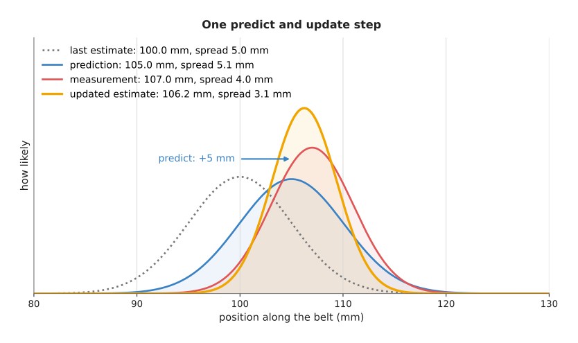
The prediction (blue) is the last estimate (dotted) moved 5 mm to the right and made a little wider. The measurement (red) is narrower than the prediction, because the camera's 4 mm spread is smaller than the prediction's 5.1 mm. That is why the updated estimate (orange) lands closer to the measurement, and it is narrower than either.
Then the table below lists all four steps of the same run, and each row is one picture.
| Step | Predicted (mm) | Predicted variance | Reading (mm) | Gain K | Updated (mm) | Updated spread (mm) |
|---|---|---|---|---|---|---|
| 1 | 105.00 | 26.00 | 107 | 0.619 | 106.24 | 3.15 |
| 2 | 111.24 | 10.90 | 109 | 0.405 | 110.33 | 2.55 |
| 3 | 115.33 | 7.48 | 118 | 0.319 | 116.18 | 2.26 |
| 4 | 121.18 | 6.10 | 121 | 0.276 | 121.13 | 2.10 |
Notice that the gain falls from 0.619 to 0.276, because as the filter becomes surer each new reading moves it less. So after four readings the spread is 2.1 mm, about half the spread of a single camera reading.
The steps as pseudocode#
The pseudocode below is the one-number filter used above, where the known change per step can be 0 for a quantity that should stay still.
function kalman_1d(readings, start_estimate, start_variance, q, r, change_per_step):
    x = start_estimate
    p = start_variance
    for each reading z in readings:
        # predict
        x = x + change_per_step
        p = p + q
        # update, only if a reading arrived
        if z is present:
            k = p / (p + r)
            x = x + k * (z - x)
            p = (1 - k) * p
        output x and p
For several numbers at once, such as a position and a speed, the same steps
use matrices. x becomes a list of numbers called the state, and p
becomes a table called the covariance, which also says how the errors of the
numbers are linked. F is the table that moves the state forward one step. H
picks out the part of the state that the sensor measures. Q and R are the
process and sensor noise as tables.
    # predict
    x = F · x
    P = F · P · transpose(F) + Q
    # update
    S = H · P · transpose(H) + R            # expected spread of the innovation
    K = P · transpose(H) · inverse(S)
    x = x + K · (z − H · x)
    P = (identity − K · H) · P
Each line matches a line of the one-number version, so S plays the part of
p + r, and the rest follows the same pattern.
The two settings: sensor noise and process noise#
Both versions of the filter need the same two settings. The sensor noise r is
the easy one, because you can measure it: hold the sensor still and record the
spread of its readings. However, the process noise q is harder, since it says
how much the quantity can change in ways the prediction does not model. It
therefore sets how quickly the filter follows real changes.
The picture below shows the difference. In it, a depth camera on the wrist reads
the distance to the table, 400 mm, with a 4 mm spread, 10 times a second.
After 3.5 seconds the arm lowers the camera by 20 mm. Then two filters run on
the same readings, one with q = 0.01 and one with q = 4.
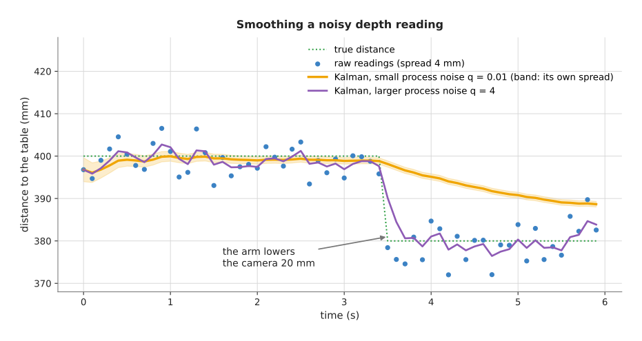
While the distance is steady, the filter with the small q is the smoother of
the two. From the 11th to the 35th reading its average error is 0.77 mm, against
1.67 mm for the other filter and 2.76 mm for the raw readings. But when the
camera drops, the small-q filter believes the distance cannot change, so it
drifts down very slowly. At the end of the run, 2.4 seconds later, it still
reads 388.7 mm, 8.7 mm too far. However, the filter with q = 4 is within 5 mm
of the new distance by the second reading after the drop.
The next picture shows why, by plotting the gain and the spread over time for the steady part.
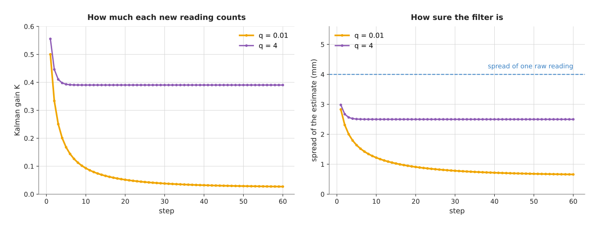
With q = 0.01 the gain keeps falling: 0.5 at the first step, 0.168 at the
fifth, 0.093 at the tenth and 0.027 at the sixtieth. As a result, the filter trusts its
own estimate more and more, and each reading counts less. This is what makes it
smooth, and also what makes it slow to follow a real change. With q = 4,
however, the gain settles at 0.39 within a few steps, and the spread settles at
2.5 mm. So that filter always gives each reading a fair share.
There is no single right q, so choose it from how fast the real quantity can
change. If you know the arm is about to move the camera, you can also tell the
filter so: the move is a known change, just like the belt's 5 mm per step.
Tracking a position and a speed together#
So far the filter has tracked one number at a time, but a part on a belt has a position and a speed. The camera measures only the position, but the filter can estimate the speed too, by putting both in its state. This is called a constant-velocity model: the predict step assumes the part keeps its speed, and adds the speed times the time step to the position. The update step corrects the position from the reading, and the covariance links position and speed, so the speed is corrected too.
The picture below tracks a part moving across a belt at about 60 mm/s, with the camera's positions scattering by 4 mm. For 0.8 seconds the arm reaches in and hides the part, so there are 8 pictures with no reading.
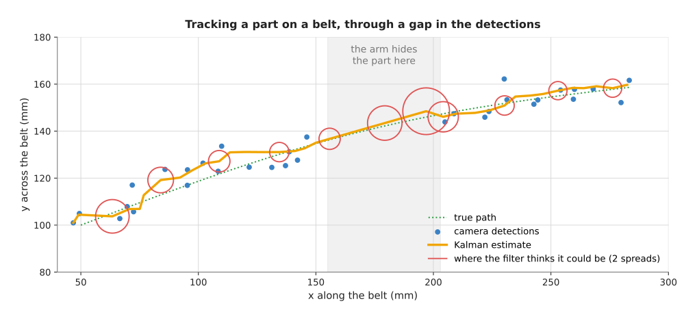
Before the gap, the filter has learned a speed of 58.7 mm/s along the belt and 16.8 mm/s across it. During the gap it keeps predicting with that speed, and the red ellipses show where the filter thinks the part could be. They grow during the gap, because there are no readings to shrink them: the spread along the belt rises from 2.0 mm to 5.0 mm. At the end of the gap the estimate is 3.6 mm from the true position, close enough to match the next detection to the same part. Then, once readings return, the ellipses shrink again.
The same growing ellipse tells a tracker how far from the prediction a new detection may be and still count as the same part. Book 2 explains this idea, called gating, in tracking and association.
The Kalman filter as described here assumes the motion and the measurement are straight-line relationships, like "position plus speed times time". However, many real problems are not, because an object turning on a turntable, or a camera measuring an angle and a distance, bends the relationship. Section 4 explains what goes wrong then, and the three filters people use instead: the extended Kalman filter, the unscented Kalman filter and the particle filter.
4. When things are not straight lines: EKF, UKF and the particle filter#
So this section is for the case the rest of the page leaves out: a motion or a
measurement that is not a straight-line relationship. It uses the same predict
and update words as section 3, and the numbers come from a real run of a second
diagram script, docs/diagrams/fitting_and_estimation_2.py.
What breaks when the relationship bends#
The Kalman filter describes what it believes as one bell curve: an estimate and a spread. That works because of one fact: push a bell curve through a straight-line relationship, such as "position plus speed times time", and you get another bell curve. As a result, the filter only has to work out its new centre and width.
However, push a bell curve through a bent relationship and the result is no longer a bell curve. Angles are the common cause of this on an arm. For example, a sensor may measure a distance and an angle, or a camera may see a turning part side-on. Then the relationship between what it reads and where the thing is becomes bent.
The picture below shows this, using a sensor that says an object is 400 mm away, give or take 5 mm, straight ahead, give or take 25°. The blue dots are 5000 positions drawn from that belief, and they form a curved band, not an oval.
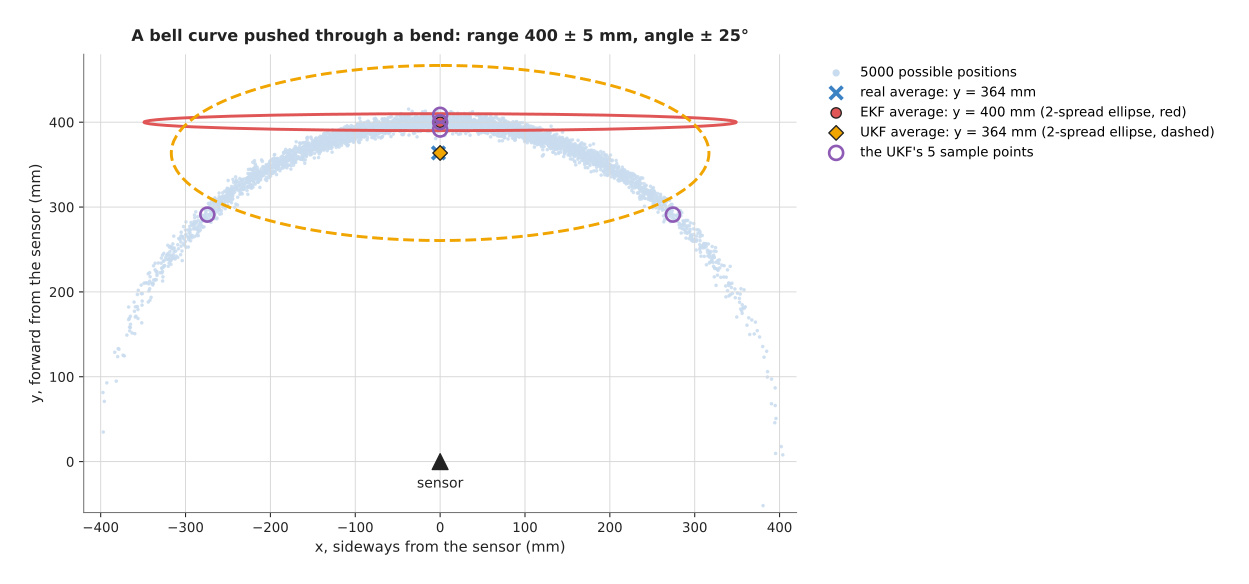
The real average of the dots is 364 mm forward, not 400 mm, because the ends of the band curve back towards the sensor. Their forward spread is 49 mm, not 5 mm, so a filter that simply converts the best guess, 400 mm straight ahead, gets both of those wrong.
The extended Kalman filter: straighten the bend at the estimate#
The first way round that problem is the extended Kalman filter (EKF), which replaces the bent relationship with a straight one that touches it at the current estimate. It is like laying a ruler against a curve at one point. The slope of that ruler is called the Jacobian: a table of how much each output changes when each input changes a little. The filter then runs the usual predict and update steps with the ruler in place of the curve.
This works well when the bend is gentle over the width of the bell curve, but badly when the bell curve is wide. In the picture, the EKF's ellipse (red) is centred at 400 mm and has a forward spread of only 5 mm. So it is sure of something that is wrong.
The unscented Kalman filter: push a few sample points through#
The unscented Kalman filter (UKF) does not straighten anything at all. Instead, it picks a small set of sample points, called sigma points, around the estimate: the estimate itself, plus two points one step out along each direction of the spread. So for two numbers that makes five points, and it pushes each point through the real, bent relationship. Then it works out a new centre and spread from where the points landed, each point with a fixed weight.
In the picture, the five purple rings are the sample points after the push. The
UKF's ellipse (dashed) is centred at 364 mm, the same as the real average, with a
forward spread of 52 mm against the real 49 mm. It still draws one oval around a
curved band, but it puts the oval in the right place and the right size. It
needs no Jacobian, so there is no slope to work out by hand. Its cost is running
the relationship 2n + 1 times per step for n numbers in the state.
The particle filter: many guesses, weighted and resampled#
Both Kalman filters still hold one bell curve, but sometimes the belief is not
one hump at all. A part seen side-on on a turntable, for example, could be at an
angle a or at the mirror angle −a: both give the same sideways position. The
belief has two humps, and one bell curve cannot hold two.
A particle filter holds the belief as a crowd of guesses instead, and each guess is called a particle. Each step then has three parts.
- Move. Push every particle through the motion model, adding a little random jitter for the process noise.
- Weigh. Give each particle a weight for how well it explains the new reading. A particle whose predicted reading is close to the real one gets a large weight.
- Resample. Draw a new crowd of the same size from the old one, where each particle is copied in proportion to its weight. Heavy particles are copied several times. Light ones die out.
The picture below shows one weigh and resample step with only 12 guesses of a part's angle, spaced 14° apart. In it, the camera read a sideways position of 122 mm. To make the bars easy to see, this picture uses a sensor spread of 15 mm rather than the 5 mm of the run below.
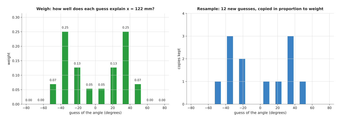
The guesses at −35° and +35° explain the reading best, with a weight of 0.25 each. After resampling they have three copies each, while the guesses at ±63° and ±77° had weights near zero and are gone. Notice that both the positive and the negative angles survive: the particle filter keeps both answers until later readings decide between them.
In pseudocode, one step looks like this:
function particle_filter_step(particles, reading):
    for each particle p:
        p = motion_model(p) + small random jitter      # move
        w[p] = how likely reading is if p were true      # weigh
    normalise w so the weights add up to 1
    particles = draw count(particles) particles, each with chance w[p]   # resample
    estimate = weighted average of the particles before resampling
    return particles, estimate
A small run: a part on a turntable#
To compare the three filters on one problem, a part sits 150 mm from the centre
of a turntable that turns at a known 0.5 rad/s. A camera looks along the table and sees only the part's sideways
position, x = 150 × cos(angle), with a spread of 5 mm, 10 times a second.
The motion is a straight line (the angle grows by 0.05 rad each step), but the
measurement is bent. The true angle starts at 37°, and the first reading is
122.5 mm.
Three filters run on the same 45 readings, and the EKF and the UKF start from a wrong guess of −34°, with a spread of 29°. That is the mirror answer, because it explains the first reading just as well. The particle filter starts with 1000 particles spread evenly all round the table, meaning it has no idea where the part is.
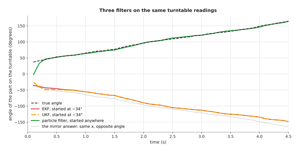
The EKF (red) and the UKF (dashed orange) both stay on the wrong side. Every reading fits the mirror angle almost as well as the true one, so each update pulls them back to it. After one second they are 121° off, and over the last three seconds they are 119° off on average. Worse, at the end they report a spread of only 1.7°: they are sure, and wrong. Started at the right angle instead, the same EKF tracks the part with an average error of 1.2°. So the EKF is fine once it is near the answer; it just cannot choose between two answers.
The particle filter (green) finds the right side within three readings. Its first estimate is 39° off, because it averages two humps and lands between them. By the third reading it is 1.3° off, and over the last three seconds its average error is 1.2°, the same as the well-started EKF.
The picture below shows why, because it draws the particles on the turntable, larger when their weight is larger.
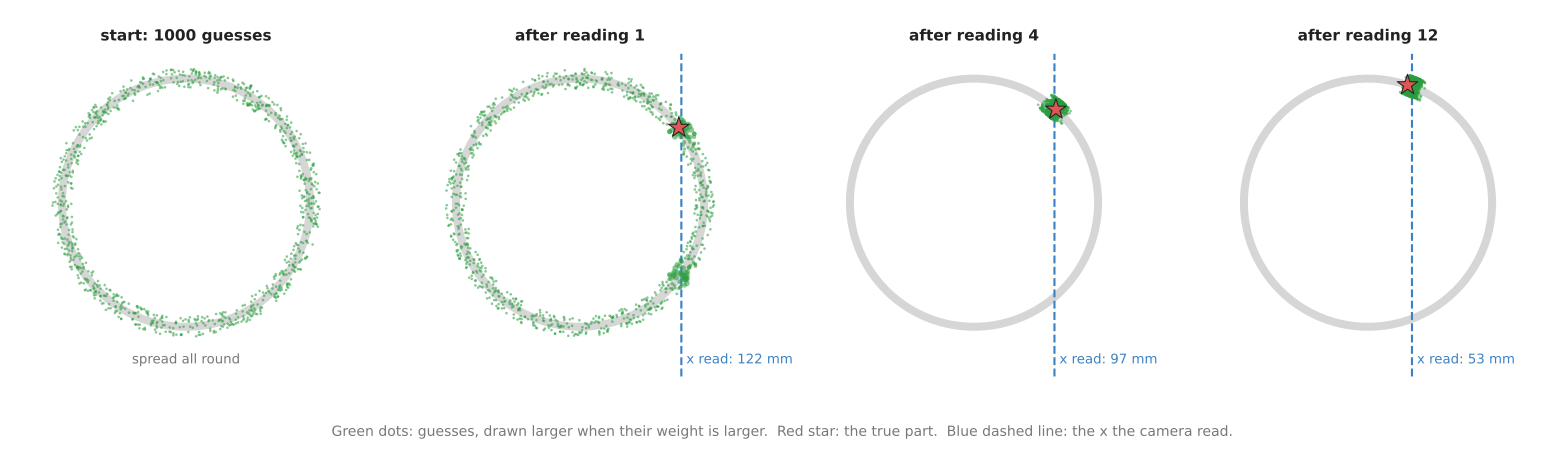
After the first reading, the weight is split almost evenly between two clusters, 48% on the mirror side and 52% on the true side. The table then turns, and on the true side the part's sideways position shrinks as the angle grows, while on the mirror side it would grow. Since the readings shrink, the mirror particles lose their weight, and by the fourth reading all the weight is on the true side.
Where each one is used, where it fails, and libraries#
Once you know how each filter behaves, it is easier to see where the three appear on a robot arm.
- EKF. Tracking an object with a camera that measures pixels, because the pinhole camera model divides by depth, which is a bend. Joining wheel counts, an inertial measurement unit and a camera on a mobile base with an arm, where headings are angles.
- UKF. The same jobs when the bend is sharper, or when working out the Jacobian by hand is error-prone.
- Particle filter. Finding where a mobile base is on a known map, where the belief often has several humps. Finding how a part sits in the hand from a few touch contacts. Deciding which of two symmetric ways round a part is, as in the turntable run.
Each has its own way to fail, so the table below gives the cause, the sign you would see, and what people do about it.
| Filter and cause | The sign you would see | What to do |
|---|---|---|
| EKF, wide spread across a sharp bend | a small spread but large, one-sided innovations; the estimate drifts | a UKF; or smaller time steps; or better starting guesses |
| EKF or UKF, two answers fit the readings | a confident estimate on the wrong answer, as in the turntable run | a particle filter at the start, then hand over to a Kalman filter |
| Particle filter, too many numbers in the state | needs far more particles; most have near-zero weight | keep the state small (up to about six numbers); use a Kalman filter for the rest |
| Particle filter, very precise sensor | all particles collapse onto a few copies, and the crowd stops exploring | more jitter in the move step; more particles |
| Particle filter, random draws | slightly different answers on every run | more particles; a fixed random seed for testing |
The Python library filterpy has ExtendedKalmanFilter and
UnscentedKalmanFilter classes, and resampling functions such as
filterpy.monte_carlo.systematic_resample, which is the resampling method this
page's script uses. The ROS 2 package robot_localization provides ekf_node
and ukf_node. The ROS 2 navigation stack, Nav2, includes nav2_amcl, a
particle filter that finds a mobile base on a map. GTSAM, listed in section 7,
handles bent relationships by re-straightening them over a window of past steps
rather than only at the latest one.
The particle filter's cost is speed, because the run above updated 1000 particles every step, where the EKF updated one number and one spread. For a small state that is still fast, but for a large one a Kalman filter that is started near the right answer is the practical choice.
5. Where it is used on a robot arm#
Whichever version of the filter is used, it appears in perception, sensing and the arm's own state.
- Tracking objects the camera sees. A tracker runs one filter per object. Each picture, it predicts every object forward, matches detections to the predictions, and updates each filter with its match. The assignment and matching page shows the matching step.
- Picking from a conveyor. The filter's speed estimate lets the arm aim for where the part will be when the gripper arrives, not where it was when the picture was taken.
- Coasting through a missed detection. When the arm hides a part, or the detector misses it for a frame, the filter keeps predicting. The growing spread tells the program when to give up on the track.
- Smoothing a depth or force reading. A wrist camera's distance to the table, or a force sensor's reading during a gentle push, is filtered before a controller acts on it. A PID controller that acts on raw readings passes the noise straight to the motors.
- Estimating a slowly changing constant. A robot that pushes objects can estimate the table's friction from push after push. The sibling repo's contact-parameters page shows that for a constant, the Kalman filter becomes recursive least squares: the least-squares fit updated one reading at a time.
- Joining sensors. A mobile base with an arm on it combines wheel counts, an
inertial measurement unit (IMU) and sometimes a camera into one position.
The ROS package
robot_localizationdoes this with an EKF or a UKF. - Estimating joint speed. An arm's encoders measure joint angles. A small filter per joint estimates the speed more smoothly than subtracting two angles and dividing by the time.
6. Where it is useful, and where it is not#
In all of those places, the filter works best when you can say how the quantity moves from one moment to the next. It also needs noise that is roughly bell-shaped and does not depend on the last reading, and readings that arrive regularly with known times.
However, the table below lists the ways it goes wrong, and each row gives the cause, the sign you would see, and what people use instead.
| What goes wrong | The sign you would see | What to use instead |
|---|---|---|
Process noise q too small | smooth but late; after a real change the estimate trails for seconds | raise q, or tell the filter about known changes such as arm moves |
Process noise q too large | the estimate is nearly as noisy as the raw readings | lower q; check with a recording of the sensor held still |
| The object stops following the motion model (a person picks it up, it hits a stop) | the estimate carries on past where the object is; innovations are suddenly large | detect large innovations and restart the track; use several motion models side by side |
| A wrong detection is fed in (the wrong object, a reflection) | a sudden jump that then decays slowly | a gate that refuses readings too far from the prediction; see tracking and association |
| Irregular timing (dropped frames, late messages) | speed estimate jumps; prediction off by one frame | use each reading's real timestamp for the time step, not a nominal rate |
| Strongly bent relationships (angles, rotations) | the filter becomes over-confident and then drifts | EKF, UKF or a particle filter, as section 4 explains; for orientation, a filter built for rotations |
| Readings with rare large errors, not bell-shaped | one bad reading drags the estimate | a gate, or a robust filter that limits the pull of one reading |
| Motion too complex to write down (a cloth, a rolling object bouncing) | large innovations all the time | a learned motion model, such as a learned dynamics model |
7. Libraries that provide it#
Since the one-number filter is ten lines of code, many projects write it themselves. For more than that, the libraries below are well known. Each row gives the library, the languages it is used from, the class or package, and a note.
| Library | Languages | Class or package | Note |
|---|---|---|---|
| OpenCV | C++, Python | cv::KalmanFilter | linear filter with the standard predict and correct steps |
| filterpy | Python | filterpy.kalman.KalmanFilter, ExtendedKalmanFilter, UnscentedKalmanFilter | readable code written alongside a free textbook on the subject |
| robot_localization | ROS 2 (C++) | ekf_node, ukf_node | joins wheel, IMU, GPS and pose readings into one position |
| GTSAM | C++, Python | factor graphs | a smoother that corrects past estimates as well as the current one; used for camera and robot position |
| Eigen | C++ | matrix types | the matrices to write your own filter with, as most C++ robotics code does |
8. Why a Kalman filter, and what it costs#
As a result, the Kalman filter is a loop that predicts a quantity forward and then corrects it with each new reading, weighting the two by how much each is trusted. It gives the arm a steady value, a measure of how sure that value is, and a prediction for the next moment, even through short gaps.
The obvious alternative is a moving average: average the last ten readings,
which is simpler and needs no model. On the steady part of the depth example, a
10-reading average has an average error of 1.08 mm, close to the Kalman filters.
However, it has three drawbacks, and the first is that it always lags. After the
20 mm drop it took seven readings to get within 5 mm, against two for the
q = 4 filter. It cannot predict ahead, so it cannot help an arm meet a moving
part. And it gives no spread, so a tracker cannot tell how far to look for the
next detection.
A second alternative is to fit a line through the last few positions with least squares and extend it forward. That gives a speed and a prediction, but it forgets everything older than its window, and it does not say how sure it is. The Kalman filter keeps all past readings in two small numbers, the estimate and the covariance, and costs the same on every step however long it runs.
The costs are these: you need a model of how the quantity moves, and the filter is only as good as that model. You must choose the process noise, and a poor choice gives either a laggy or a noisy result without any error message. The filter's confidence is highest just before an object does something new, such as change direction. And its state lives on from step to step, so a wrong reading or a bug can affect many steps after it.
9. The learned alternative#
Those costs raise the question of a learned alternative, but the learned trackers in Book 7's tracking and motion mostly keep the filter rather than replace it. Methods such as SORT and ByteTrack take boxes from a trained detector and use a Kalman filter to predict where each object should be, and some also compare how the objects look, so that two similar objects are not swapped. When the motion is too complex to write down, a learned dynamics model predicts the next state from recordings of the real arm instead of a formula, but it needs those recordings, and its errors add up over many steps. For touch, force and slip models recognise patterns such as the fast shaking of a slip, which a filter that smooths the reading cannot tell apart from noise. For a steady estimate of a position or a speed, the Kalman filter is still the better choice, because it needs no training data, costs a few lines of arithmetic per reading, and says how sure it is.
10. Where to read next#
The pages below cover what this filter builds on, and where its output is used.
- Least-squares fitting is the batch version of the same idea. For a quantity that does not change, the Kalman filter gives the least-squares answer one reading at a time.
- RANSAC handles bad points in a batch. A gate does the same job for a filter.
- Assignment and matching matches new detections to the filter's predictions.
- PID control often acts on a filtered reading.
- Book 2 goes deeper into tracking on a real arm in tracking and association.
11. Using it in Python#
Section 3 worked through the belt example by hand, and section 7 named filterpy as the library that does the same arithmetic for more than one number at a time. This section shows that library on the same belt, so you can compare the code with the table in section 3. After it you will be able to run a filter that tracks a position and a speed together, and you will know exactly which of its settings describe your robot rather than the filter.
The program below is the belt example from section 3, with the state holding both the block's position and its speed as in the last part of that section. filterpy is a small library whose classes hold the matrices as plain attributes, which makes it easy to see the correspondence with the steps on this page.
import numpy as np
from filterpy.kalman import KalmanFilter
from filterpy.common import Q_discrete_white_noise

dt = 0.1                                  # the camera gives 10 pictures a second
kf = KalmanFilter(dim_x=2, dim_z=1)       # state: position and speed; one reading
kf.x = np.array([100.0, 50.0])            # start: 100 mm, moving at 50 mm/s
kf.F = np.array([[1.0, dt],               # predict: position += speed * dt
                 [0.0, 1.0]])             #          speed stays the same
kf.H = np.array([[1.0, 0.0]])             # the camera sees position, not speed
kf.P = np.diag([25.0, 100.0])             # how unsure the start is, as variances
kf.R = np.array([[16.0]])                 # camera noise: a 4 mm spread, squared
kf.Q = Q_discrete_white_noise(dim=2, dt=dt, var=100.0)   # process noise

for reading in (107.0, 109.0, 118.0, 121.0):
    kf.predict()
    kf.update(reading)
    print(kf.x[0], kf.x[1], np.sqrt(kf.P[0, 0]), kf.mahalanobis)
Run it and the four steps print 106.24, 110.32, 116.26 and 121.25 mm, with the spread falling from 3.15 mm to 2.39 mm. The first of those matches the 106.24 mm in the table in section 3 exactly, because it is the same arithmetic. The speed estimate stays between 49.3 and 51.2 mm per second, which brackets the real belt speed even though no reading measures speed at all.
The library does the predict and update matrix arithmetic, and it also gives you
two things the hand-worked example did not. kf.y is the innovation, the
difference between the reading and the prediction, and kf.mahalanobis is that
difference measured in units of the spread. That second number is the gate
described in section 6: a value above about 3 means the reading is further off
than the filter's own uncertainty can explain, so you skip the update call and
let the prediction carry on alone. Q_discrete_white_noise also builds the
process noise matrix for you from one number, which saves writing out the
correlation between position and speed by hand.
What you still have to write is the model, and this is the sentence to remember
from the whole page. kf.F says how the quantity moves when nothing measures
it, kf.H says how your sensor relates to the quantity, and both of those are
statements about your robot that no library can guess. A belt gets the F
above, while a part sitting still gets an F of all ones with no speed, and a
wrist camera reading a distance through a lens gets an H that is not a plain
- You also write the loop, the gate, and the handling of a missing reading,
which is simply calling
predictwithoutupdate.
What you have to decide or measure are the four matrices of numbers. kf.R you
measure, by holding the sensor still and recording the spread of its readings,
then squaring that spread. kf.P is your honesty about the first guess, and
setting it too small makes the filter ignore the first few real readings. kf.Q
is the hard one, because section 3 showed that it sets how quickly the filter
follows a real change, and there is no measurement that gives it to you. You
choose it from how fast the quantity can genuinely move, and you check the
choice by running the filter on a recorded trace and looking at whether it lags.
Finally you decide dt, and it must be the real time between readings rather
than the rate you hoped for, which is why the
sensor streams page insists on reading the time stamp on
every message.