This chapter is about getting a clean shape or a steady number out of noisy measurements. This is difficult because every sensor on a robot arm gives readings that are a little wrong. For example, a depth camera's points scatter a millimetre or two either side of the real surface. A detector's box jumps by a few pixels from one picture to the next, and a force sensor's reading shakes even when nothing touches it. That is why the techniques in this chapter take many such readings and give back one answer that is better than any single reading.
This page is for a reader who knows what a point cloud, a camera frame and a joint angle are, as Books 1 and 2 explain, but who has not met these techniques before. It says what the chapter's five technique pages cover, which question each one answers for an arm, how they compare, and how they connect to the rest of this book and to the learned models in Book 6.
Contents#
- What fitting and estimation are for
- The question they answer for an arm
- The techniques, in two groups
- How they compare
- How this chapter connects to the others
- Where to read next
- Using it in Python
1. What fitting and estimation are for#
Fitting and estimation are the two ideas named in the chapter's title, and they are easiest to understand one at a time. Fitting means choosing the shape that best matches a set of measured points, and that shape is described by a few numbers. For example, a line has a slope and an offset, while a plane has a direction it faces and a distance from the origin. Once again, a circle has a centre and a radius. So fitting finds the values of those numbers that put the shape as close as possible to all the points at once.
Estimation means working out a number you cannot measure directly, or cannot measure without noise, from the readings you do have. For example, a camera watching a part on a moving belt gives a slightly wrong position in every picture, and sometimes no position at all. Estimation therefore combines those pictures over time into one position that is steadier than any single picture.
The two ideas overlap, because fitting a line to points is itself an estimate of the line's slope and offset. So what separates them is mostly how the data arrives. Fitting usually takes a batch of points measured at one moment. Instead, estimation over time takes one reading after another, and it updates its answer as each one arrives.
An everyday example shows the same core idea at work. Suppose you weigh a bag of flour five times on a kitchen scale and get 1003 g, 998 g, 1001 g, 997 g and 1002 g. You would not trust any one reading, so you would take the average, 1000.2 g. That average is the simplest possible fit, because it is the single number closest to all five readings. Every technique in this chapter is a more careful version of that average.
For example, the picture below shows three of the jobs this chapter covers, on made-up but realistic data.
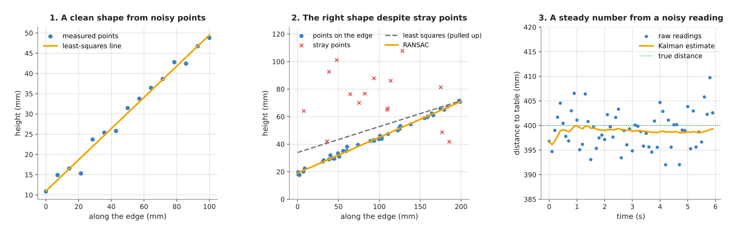
On the left, a least-squares line passes through the middle of 15 noisy points. In the middle, a random sample consensus (RANSAC) line follows the real edge, while a least-squares line through the same points is pulled upwards by the stray points. On the right, a Kalman filter turns a depth reading that shakes by about 4 mm into an estimate that stays within a millimetre or so of the true 400 mm.
2. The question they answer for an arm#
Those two definitions come together on an arm, where fitting and estimation answer a single question: given these noisy readings, what is really there, and how sure can I be?
An arm needs clean numbers because it acts on them, so a small error in a number becomes a physical mistake. For example, a gripper that closes 3 mm to the side of a glass knocks it over. In the same way, a camera that believes the table is 2° tilted when it is level puts every object at the wrong height. Because the arm cannot wait for a perfect sensor, it has to make the best of the readings it already has.
So the list below gives typical places on an arm where the question comes up.
- Finding the table in a depth camera's point cloud, so that everything that is not table can be treated as an object.
- Measuring the centre and radius of a cup or a glass from the part of its rim the camera can see.
- Finding which way the flat face of a box points, so the gripper can line up with it.
- Following a part on a conveyor belt, so the arm can meet it at the right place, even when the arm's own body hides it from the camera for a moment.
- Smoothing a force or depth reading before a controller acts on it, and pairing it in time with the camera frame it belongs to.
- Measuring the numbers in the arm's own physics, such as a joint's friction or the mass of the part in the gripper, from how the arm responds to a planned move.
- Working out a calibration, such as where the camera sits on the arm, from many pairs of measurements. The calibration page covers that case.
The picture below shows two of these jobs on one simulated table scene.
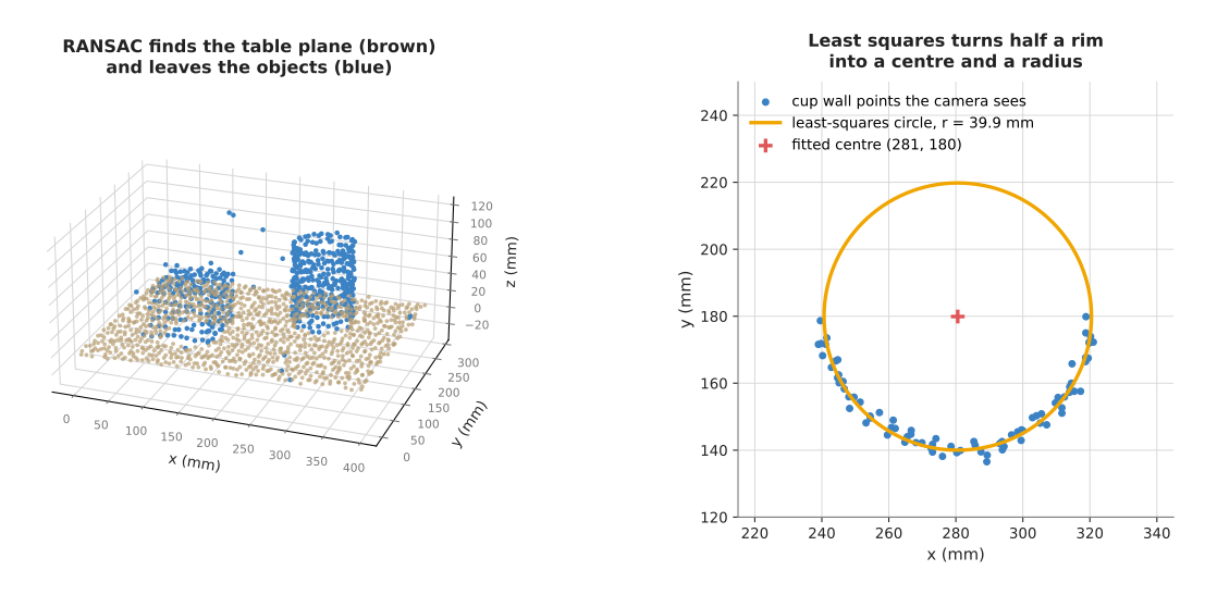
On the left, RANSAC finds the table plane among 1669 points from a depth camera (brown) and leaves 549 points on a box, a cup and a few stray readings (blue). On the right, a least-squares circle fitted to the 79 cup-wall points that face the camera gives a centre within 1 mm of the true one and a radius of 39.9 mm for a cup that is 40 mm in radius.
3. The techniques, in two groups#
Because that one question comes up in so many places, the chapter answers it on five technique pages. Each page takes a slightly different version of the question, and the five are split into two groups by how often an arm runs them. The most used group holds the four techniques that nearly every arm with a camera or a sensor runs, often on every frame. The also used group holds a technique that matters a great deal when it is needed, but that an arm runs less often. It comes up when the arm is set up, when it picks up a new part, or while it warms up.
The most used group, in 02_most-used/, holds these four pages:
- Least-squares fitting finds the line, plane or circle that is closest to all the points, where "closest" means the sum of the squared distances is as small as possible. It is fast, exact and has no settings to tune, but it assumes every point belongs to the shape.
- RANSAC, short for random sample consensus, finds the shape that the largest number of points agree with. It tries many shapes, each through a few randomly chosen points, and keeps the one with the most points close to it, so it copes with data where a third or even half of the points belong to something else.
- The Kalman filter keeps a running estimate of a changing quantity, such as the position and speed of a moving part. At each new reading it first predicts where the quantity should be, then corrects the prediction with the reading, and it also keeps track of how sure it is. Its section 4 covers the extended and unscented Kalman filters and the particle filter, for motions and measurements that are not straight-line relationships, such as angles.
- Sensor streams covers the timing and filtering of sensor data before any of the other techniques sees it: pairing readings from two sensors that were taken at nearly the same time, allowing for the delay between a measurement and its arrival, smoothing with low-pass and median filters, working out how fast a reading is changing, and switching on a threshold without flickering, using two limits (called hysteresis).
The also used group, in 03_also-used/, holds one page:
- System identification measures the numbers inside a physical model of the arm, such as a joint's friction, a payload's mass or a finger's stiffness. It plans a probe move that makes each number show up, fits the numbers by least squares, follows numbers that drift with recursive least squares, and states an error bar for each one, so the arm can act on the cautious end of the range.
In practice the techniques are often used together, as a typical table-top pipeline shows. That pipeline first lines up each depth picture with the arm's joint readings from the same moment, as the sensor streams page explains. It then runs RANSAC to find which points belong to the table, and after that least squares on just those points to get the most accurate plane. Later, a Kalman filter smooths the position of each object from picture to picture. System identification sits underneath all of this, because it gives the controller the friction and payload numbers it needs to move the arm accurately.
4. How they compare#
Since the five pages answer such different versions of the question, the table below compares them side by side. Read each row as one property and each column as one technique. The first four columns hold the most used group, and the last column holds the also used group.
| Property | Least squares | RANSAC | Kalman filter | Sensor streams | System identification |
|---|---|---|---|---|---|
| What goes in | a batch of points | a batch of points, some of them wrong | one reading at a time, over time | raw readings from several sensors, each with a time stamp | readings recorded during a planned probe move, or during normal work |
| What comes out | the numbers of a shape, and how far the points sit from it | the numbers of a shape, and which points agree with it | the current value, and how uncertain it is | readings lined up in time, smoothed, with slopes and on/off decisions | the numbers in a physical model, each with an error bar |
| Copes with stray points | no; one bad point pulls the answer | yes, up to about half the points or more | only if a gate throws them away first | a median filter removes single spikes | no, unless large residuals are thrown away |
| Settings to choose | none | a distance limit and a number of tries | how noisy the sensor is, and how much the quantity can change | how far apart two readings may be in time, filter strengths, threshold limits | the probe move; for drifting numbers, a forgetting factor |
| Same answer every run | yes | no, it uses random choices | yes (the particle filter uses random choices) | yes | yes |
| Speed | very fast, one direct calculation | slower, many tries | very fast per reading; a particle filter is slower | very fast per reading | fast to fit; the probe move takes time on the arm |
| Typical arm use | plane, line and circle measurement; calibration | finding the table; shapes in cluttered clouds | tracking a moving part; smoothing a sensor | pairing a camera frame with joint angles; detecting contact from a force reading | joint friction; payload mass; a finger's stiffness |
5. How this chapter connects to the others#
The table shows what each technique does on its own, but none of them works alone. This is because fitting and estimation sit between the raw sensor and the decisions the arm makes. This means the chapter takes ideas from earlier chapters and feeds its results to later ones.
- From geometry and cameras it takes the step that turns pixels and depths into 3D points, so every fit in this chapter starts from points that the pinhole camera model produced.
- From searching and matching it takes the nearest points around each point, which is how a surface's direction is found at each point. Iterative closest point runs a least-squares fit inside every one of its steps, and a Kalman filter's prediction is what assignment and matching compares new detections against.
- It hands the points left over after the table is removed to clustering, which splits them into objects.
- In planning and search, numerical inverse kinematics solves a least-squares problem at every step, as the page on numerical inverse kinematics explains.
- In control and motion, a controller such as PID often acts on a filtered reading rather than the raw one. The equations of arm dynamics contain the masses and friction numbers that system identification measures.
Book 6 covers learned models that do some of the same jobs in a different way. For example, a point cloud model can label which points are table and which are object, and a keypoint and pose model can give an object's position and direction directly from a picture. A learned tracker, described in tracking and motion, can follow objects that a constant-speed model cannot. However, the written techniques in this chapter need no training data, give the same answer for the same input (apart from RANSAC's random choices), and state how far off they might be. The learned models, in return, handle shapes and movements that are hard to write down as a few numbers. That is why many arms use both: a model finds the object, and a fit measures it.
Even the learned models rest on this chapter, because training a neural network means making the sum of its squared errors, or a similar number, as small as possible. That is the same idea as least squares, as the page how a model learns explains.
6. Where to read next#
Once you know what each technique is for, the order below is the one to read the pages in.
- Start with least-squares fitting. The other pages build on it.
- Then read RANSAC, which makes fitting safe when some points are wrong.
- Then read the Kalman filter, which moves from one batch of points to readings that arrive over time.
- Then read sensor streams, which prepares readings in time before any fit or filter uses them.
- Read system identification when the arm needs the numbers of its own physics, such as friction or a payload's mass.
- The map of techniques shows where this chapter sits among the seven categories in this book.
- The building blocks explains noise and uncertainty, which this whole chapter is about.
- Book 2 shows these techniques at work on real perception tasks in methods you write yourself and tracking and association.
7. Using it in Python#
Section 1 said that fitting takes a batch of points measured at one moment, while estimation over time takes one reading after another as it arrives. That difference shows up directly in the code, because the two halves of this chapter are called in two different ways. After this section you will be able to run both kinds of call on the same readings, and you will know which lines a library writes for you and which lines you have to supply yourself.
The program below uses the five weighings of flour from section 1. It first fits a straight line through them with NumPy, which is the array library that nearly all Python robotics code is built on. It then feeds the same five readings one at a time to a Kalman filter from filterpy, which is a small library of filters written alongside a free textbook on the subject.
import numpy as np
from filterpy.kalman import KalmanFilter

grams = np.array([1003.0, 998.0, 1001.0, 997.0, 1002.0])

# The batch fit: one line through all five readings at once.
slope, offset = np.polyfit(np.arange(grams.size), grams, deg=1)

# The same readings as a stream, one at a time.
kf = KalmanFilter(dim_x=1, dim_z=1)
kf.x = np.array([1000.0])   # first guess for the weight
kf.F = np.array([[1.0]])    # the weight does not change between weighings
kf.H = np.array([[1.0]])    # the scale reads the weight directly
kf.P = np.array([[25.0]])   # how unsure that first guess is, as a variance
kf.R = np.array([[9.0]])    # how noisy one weighing is, as a variance
kf.Q = np.array([[0.0]])    # nothing disturbs the bag between weighings
for g in grams:
    kf.predict()
    kf.update(g)
Run that and the fit gives a slope of −0.3 g per weighing and an offset of 1000.8 g. That slope is small next to the 2.3 g spread of the five readings themselves, so there is no real trend here. The filter ends at 1000.19 g with a spread of 1.30 g, which is the same answer as the plain average of 1000.2 g. That agreement is not a coincidence, because for a quantity that does not change the Kalman filter is the least-squares fit worked out one reading at a time.
What the libraries do for you is the arithmetic. np.polyfit builds and solves
the linear system behind the fit, and KalmanFilter does the matrix multiplies
of the predict and update steps. Neither is long, but both are easy to get
subtly wrong by hand, and both are already tested.
What you still have to write is everything around the call. You have to collect the readings, decide which shape or which model you are fitting, and check the result before acting on it. In the fit that means looking at how far the points sit from the line, and in the filter it means watching the spread and rejecting a reading that is much further off than the spread allows.
What you have to decide or measure is the part no library can supply. The fit
needs you to choose the shape, because deg=1 asking for a line is your claim
about the data and not a fact NumPy checked. The filter needs three numbers from
you: the first guess kf.x, how unsure that guess is in kf.P, and the sensor
noise in kf.R, which you get by holding the sensor still and recording the
spread of its readings. It also needs kf.Q, the process noise, which says how
much the quantity can change in ways the model does not describe, and that one
you have to reason about rather than measure. Every page in this chapter ends at
the same place, with a short library call wrapped around numbers that describe
your own robot.