This page explains how to work with a stream of sensor readings. This means readings that arrive one after another, many times a second, for as long as the arm runs. It answers the five questions that come up most often once you write a program against such a stream. How do you pair a camera picture with the joint angles of the same moment? What goes wrong when two devices keep their own clocks? How do you smooth a noisy reading, and what does smoothing cost? How do you get a rate of change, such as how fast a force is rising, out of noisy readings? And how do you turn a reading into a yes-or-no flag, such as "the force is too high", without the flag flickering on and off?
It is for a reader who knows what a joint angle, a wrist camera and a force
sensor are, at the level of Books 1 and 2. So this page does not explain those
parts again. It also helps to have read the
Kalman filter page, because that page handles one stream
in a more careful way than anything here does. Every number on this page comes
from a real run of the diagram script,
docs/diagrams/sensor_streams_and_safety.py, rather than from an estimate.
Two running examples are used throughout, and both come from an ordinary arm. The first is a wrist camera, which is a camera fixed to the arm near the gripper, so that it moves whenever the arm moves. The second is a force-torque trace, which is the stream of readings from a force-torque sensor at the wrist. That means a stream of numbers saying how hard the tool is pushing on something.
Contents#
- What this page answers
- The idea in one sentence
- How it works, step by step · Every reading carries a time stamp · Pairing a picture with the arm's pose · Clock offsets and latency · Smoothing: moving average, exponential and median filters · A slope from noisy readings · Thresholds that do not flicker: hysteresis and debouncing · The steps as pseudocode
- Where it is used on a robot arm
- Where it is useful, and where it is not
- Libraries that provide it
- Why these techniques, and what they cost
- The learned alternative
- Where to read next
- Using it in Python
1. What this page answers#
A robot arm has many sensors, and each one sends its own stream at its own rate. The joint encoders report the joint angles perhaps 100 or 1,000 times a second, and an encoder is the sensor inside a joint that measures its angle. A wrist camera is much slower, because it sends only 30 pictures a second, while a force-torque sensor is faster again at 500 or 1,000 readings a second.
Because those rates differ, and because no reading is perfect, these streams cause four everyday problems.
- The streams do not line up, because a picture is taken between two joint readings rather than at the same instant as one.
- Every reading is late, so a picture arrives at the computer some tens of milliseconds after it was taken.
- Every reading is noisy, since a force sensor's reading shakes a little even when nothing touches it, and now and then it jumps for no real reason.
- Decisions made from noisy readings flicker, so a check such as "is the force above 10 newtons?" can switch between yes and no hundreds of times while the real force sits near 10.
The techniques on this page are small, and none of them needs a model of the arm, but almost every arm program uses all of them. Getting them wrong causes some of the hardest bugs to find, because nothing crashes. Instead the arm just places things a few millimetres off, or stops for no visible reason.
2. The idea in one sentence#
Since the four problems above all come from time, the answer is stated in terms of time as well.
Treat each reading as a value together with the moment it was true, combine readings by their moments rather than by when they arrived, and smooth and threshold them in ways whose delay you have measured.
Here is an everyday example of the same rule, taken from outside robotics. You take a photo from a moving train, while a friend on the train writes down where the train is every second. Later you want to know where each photo was taken, so you must match each photo to one of the positions your friend wrote down. You do not use the position written down at the moment you looked at the photo, because that moment has nothing to do with the photo. Instead you use the position at the time printed on the photo. So if the photo says 10:15:03.5, you take the positions at 10:15:03 and 10:15:04 and pick the point halfway between them. And if your camera's clock is a minute fast, you must correct for that first, or every photo is placed a minute's travel down the line.
3. How it works, step by step#
Every reading carries a time stamp#
That rule starts from the moment a reading was true, so the first thing every stream needs is a way of writing that moment down. A time stamp is the moment a reading was true, recorded together with the reading itself. In the Robot Operating System (ROS), most messages carry a header. This header holds the time stamp and the name of the frame the numbers are measured in. Book 4's ROS introduction shows the header, while Book 2's section on the right frame at the wrong instant shows what goes wrong without it.
The rule about stamps is short, and it decides everything that follows: the time stamp should say when the reading was true, not when it arrived. For a picture that is the moment the camera's sensor was exposed to light, and for a force reading it is the moment the sensor sampled. So a program that uses the time its callback ran, instead of the stamp, is using the arrival time. Here the callback is the function that runs when a message arrives.
Pairing a picture with the arm's pose#
Once every reading carries a stamp, two streams can be paired by those stamps, and the picture below shows the two streams of the running example. The joint angles arrive 100 times a second, while the wrist camera takes only 30 pictures a second. The arm moves the tool 100 mm in 0.6 seconds along a smooth path. As a result, at the moment of the marked picture the tool is moving at 261 mm/s.
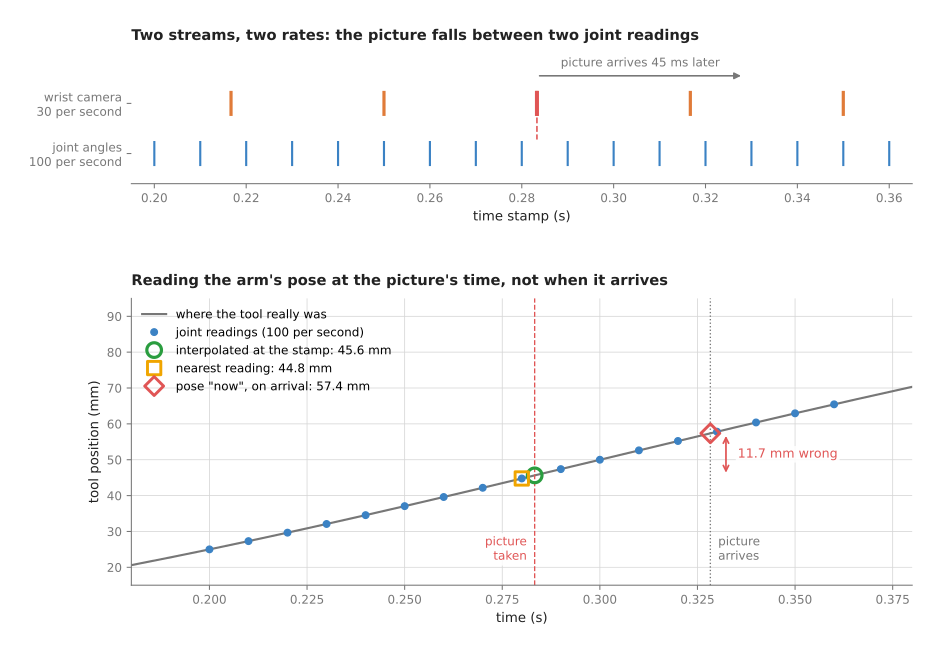
The picture has the time stamp 0.2833 s, which falls between the joint readings at 0.28 s and 0.29 s. So there are three ways to get the arm's pose for it.
- Read the pose "now", when the picture arrives. The picture arrives 45 ms after it was taken, so by then the tool is at 57.4 mm although it was really at 45.6 mm. That means the pose is 11.7 mm wrong, and this is the most common mistake of the three.
- Take the nearest joint reading. The nearest one is at 0.28 s, which is 3.3 ms before the picture, and it gives 44.8 mm, so the error is 0.9 mm. At 100 readings a second the nearest reading is never more than 5 ms away, so at this speed the error is never more than about 1.3 mm.
- Interpolate at the picture's stamp. Interpolate means working out a value between two known ones, here by drawing a straight line between the readings at 0.28 s and 0.29 s. It gives 45.6 mm, which is the same as the true position to one decimal place.
Method 2 is called approximate-time matching, because it pairs each message
with the message from the other stream whose stamp is closest. ROS provides it as
ApproximateTimeSynchronizer in the message_filters package, which Book 2's
one-box code
introduces. You give it a slop, which is the largest difference between two
stamps that still counts as a pair. That is why the method suits two streams at similar
rates, such as a colour picture and a depth picture.
Method 3 suits a slow stream against a fast one instead, such as pictures against
joint angles. Keep the last second or so of joint readings in a buffer. Then,
when a picture arrives, look up the two readings either side of its stamp and
interpolate between them. This is exactly what the ROS transform library, tf2,
does when you ask lookup_transform for the pose at a given time. Book 2's
wrist camera page
does this in its code, where the rule is written as "the pose must belong to the
frame, not to now".
Clock offsets and latency#
Pairing by stamps only works when the stamps themselves are right, and two different delays hide in a stream, so each one needs its own fix.
Latency is the time between a reading being true and it arriving, and for the camera above it is 45 ms. It comes from the exposure, the transfer over the cable, and the driver's work. Latency on its own is harmless if the stamp is right, because you look up the pose at the stamp. So it only matters when you act on the result, since an arm steering by a picture is always steering by the past.
A clock offset is a difference between two clocks. Such an offset appears because the camera may stamp its pictures with its own internal clock, while the joint readings are stamped with the computer's clock. If the camera's clock runs 12 ms ahead, every picture looks 12 ms later than it was. So in the example, pairing by the uncorrected stamp gives the pose at 0.2713 s instead of 0.2833 s. That is 42.5 mm instead of 45.6 mm, which is 3.1 mm wrong. Nothing warns you, because the pairs look perfectly matched.
Clocks also drift, which means that two clocks agreeing at start-up slowly move apart, because no two crystals tick at exactly the same rate. So an offset measured once is not enough for a long run.
Three fixes are used against these clock problems, and the most reliable comes first.
- Put every device on one clock. Computers are kept in step with the Precision
Time Protocol (PTP), which some cameras and arm controllers also support, or
with the Network Time Protocol through a program such as
chrony. - Let the driver translate, because some camera drivers convert the camera's own time into the computer's time. The Intel RealSense library, for example, has a "global time" setting that does this.
- Measure the offset yourself by moving the arm at a steady speed past a marker the camera can see. Then find the time shift that makes the marker's position in the pictures agree best with the arm's recorded position. That shift is the offset, together with any stamping delay in the driver.
Smoothing: moving average, exponential and median filters#
Correct stamps put every reading at the right moment, but they do nothing about noise, so the next step is to smooth each stream. A filter here is a small calculation that takes the stream of raw readings and gives back a smoother stream. Filters that let slow changes through and damp fast ones are called low-pass filters. The PID page uses one to clean up a noisy speed.
The picture below uses the force-torque trace, where the sensor sends 500 readings a second with 0.25 N of noise. The tool moves freely until 0.5 s and then touches a surface, so the force rises at 20 N/s to 6 N and stays there. Three single-reading spikes of +4 N stand for electrical glitches, and three filters run on the same raw readings.
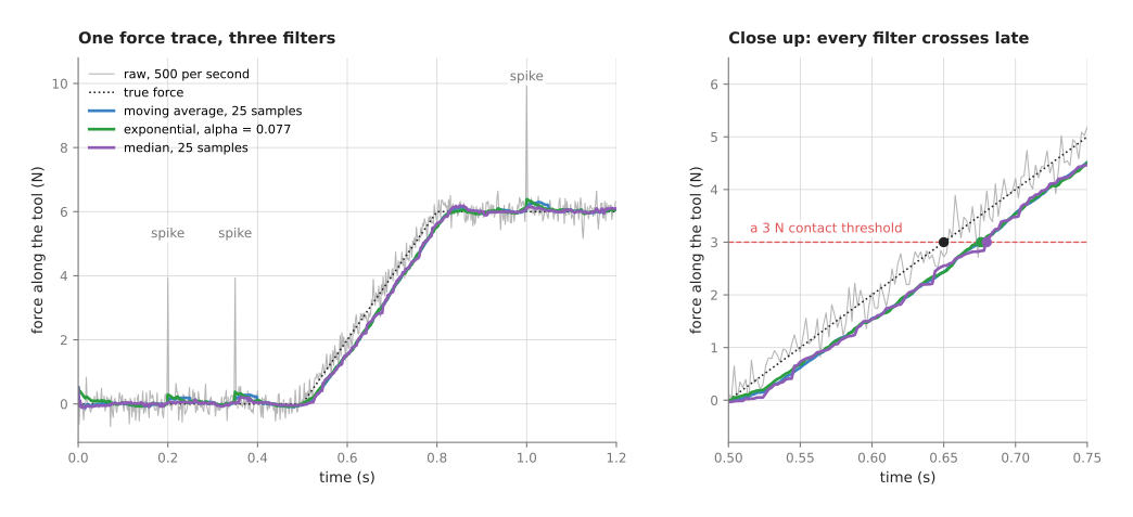
- A moving average reports the average of the last
nreadings, and herenis 25, which is 50 ms of readings. On the quiet part before contact it cuts the spread of the readings from 0.25 N to 0.04 N. A spike of 4 N becomes a bump of about 0.3 N, because the spike is shared among 25 readings. - An exponential filter keeps one number, the estimate, and each new reading
moves the estimate a fixed fraction of the way towards itself:
estimate = estimate + alpha × (reading − estimate). Herealphais 0.077, which is the usual match for a 25-reading average. That is why it behaves much like the moving average, with a spread of 0.055 N and a spike bump of about 0.4 N. It needs no buffer of past readings, which is why it is popular on small processors. - A median filter reports the middle value of the last
nreadings once they are sorted. It has a spread of 0.04 N, and the spikes almost vanish, because the worst bump is 0.2 N, which is the noise itself. A single wild reading only moves the median by one place in the sorted list. Book 2's section on conditioning a force reading explains this with a 200 g object and a 9,577 g spike.
Every filter is late, however, and the right panel shows the moment each output
first crosses 3 N. The true force crosses at 0.650 s, while the moving average
and the exponential filter cross at 0.676 s, 26 ms late. The median crosses at
0.680 s, which is 30 ms late. A causal moving average of n readings is late by
about half its window, here 12 readings or 24 ms. The word causal means that
it uses only readings that have already arrived, as any filter on a running robot
must.
The raw readings are not late, but they cannot be used either. A 3 N threshold on the raw readings would have fired at 0.20 s on the first spike, while the tool was still in free air.
This is the trade that runs through every filter, since a longer window gives a smoother signal and a later one. Choose the window from the noise you must remove and the delay you can afford, and measure both.
A slope from noisy readings#
Smoothing gives a steadier value, but often the useful number is how fast a reading changes rather than the reading itself. How fast the force rises tells you how stiff the surface is, and how fast a joint angle changes is the joint's speed. This rate of change is called the derivative, or the slope.
The obvious way is to subtract neighbouring readings and divide by the time between them, and the picture below shows why that fails. It uses the rising part of the force trace, where the true slope is 20 N/s.
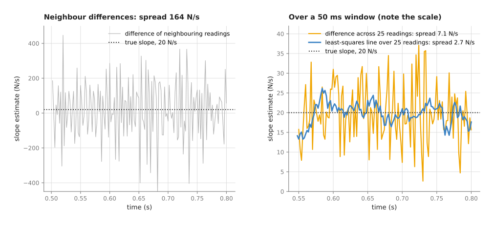
The readings are only 2 ms apart, so noise of 0.25 N divided by 0.002 s is already 125 N/s. As a result the neighbour differences have a spread of 164 N/s around a true value of 20 N/s. Their average is right at 20.2 N/s, but no single value is any use.
Two better ways use a window of 25 readings, which is 50 ms long.
- The difference across the window subtracts the reading 25 places back, so the noise is the same while the time between the two readings is 25 times longer. That brings its spread down to 7.1 N/s.
- A least-squares line through all 25 readings uses every reading in the window rather than just the two ends, and least-squares fitting explains how. Its slope has a spread of 2.7 N/s, and its average is 19.8 N/s.
Both are late by about half the window, 24 ms, for the same reason as the filters. A Kalman filter that tracks a value and its speed together, as on the Kalman filter page, is the next step up. The Savitzky–Golay filter in SciPy fits a small curve in a sliding window and can return its slope, which is the same idea as the least-squares line.
Thresholds that do not flicker: hysteresis and debouncing#
Once a value is smooth and its slope is known, the last step is to turn it into a decision. A threshold does that by turning a reading into a flag, so that "the force is above 10 N" is either true or false. The trouble comes when the real value sits near the threshold, because noise then pushes each reading to one side or the other at random.
The picture below shows a force that climbs to 9.8 N, creeps up to 10 N, rises to 11.5 N, then falls back to 6.5 N. In that run the noise is 0.3 N and the limit is 10 N.
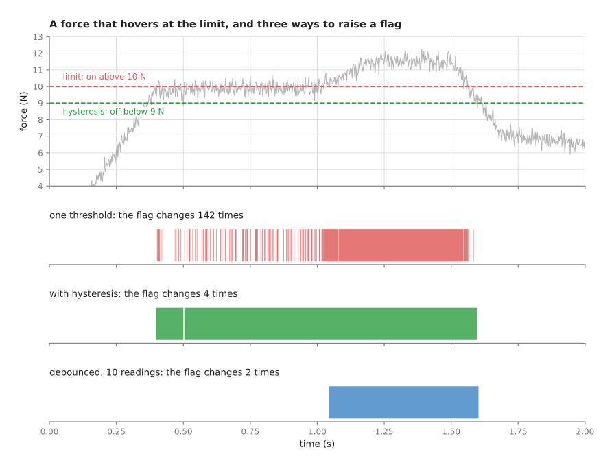
- One threshold. The flag is on whenever the reading is above 10 N, and it changes 142 times in two seconds. So a program that stops the arm when the flag goes on, and restarts it when the flag goes off, would jerk the arm about.
- Hysteresis. The flag turns on above 10 N but only turns off below 9 N, because hysteresis means that the switch-on level and the switch-off level are different, so the flag remembers which side it came from. The gap between the two levels must be wider than the noise. Here it changes 4 times, since the gap of 1 N is only about three times the noise, so one dip early on still gets through. A wider gap between the two levels would remove that dip.
- Debouncing. The flag only changes after 10 readings in a row, 20 ms, agree with the new state, and the word comes from mechanical switches, whose contacts bounce open and shut for a moment when pressed. Here the flag changes twice, on at 1.044 s and off at 1.602 s. That is because it ignored the early touches of 10 N, when the real force was still 9.8 N, and waited until the real force was clearly above the limit.
The two tricks do different jobs, and they are often used together. Hysteresis stops the flag chattering once it has changed, while debouncing stops a brief excursion from changing it at all. But debouncing adds a delay, because here the flag waits 20 ms before acting. For a safety stop that delay must be counted, and it should be short. Instead, for a slow decision such as "the part is seated", a longer wait is fine. The edges and contours page uses the same two-level idea to link edge pixels.
The steps as pseudocode#
All five steps sit in one program, so the pseudocode below puts them in the order they run. That order is to pair the streams, smooth them, take a slope, and then set the flag.
# 1. pair a slow stream with a fast one
pose_buffer = ring buffer of (stamp, joint_angles), last 1 second
on joint reading (stamp, angles):
    append (stamp, angles) to pose_buffer
on picture (stamp, image):
    stamp = stamp - camera_clock_offset           # measured, or zero if on one clock
    before, after = readings either side of stamp in pose_buffer
    if none, or the gap between them > 2 × joint period:
        drop the picture and count it              # never fall back to "now"
    w = (stamp - before.stamp) / (after.stamp - before.stamp)
    angles = before.angles + w × (after.angles - before.angles)
    use (image, angles) together

# 2. smooth, and 3. take a slope, over the last n readings
window = last n readings
smooth = median(window)                            # or mean, or an exponential filter
slope  = slope of the least-squares line through (stamps, window)

# 4. a flag with hysteresis and debouncing
if flag is off and smooth > on_level:  count_up = count_up + 1  else count_up = 0
if flag is on  and smooth < off_level: count_down = count_down + 1 else count_down = 0
if count_up   >= k: flag = on,  count_up = 0
if count_down >= k: flag = off, count_down = 0
4. Where it is used on a robot arm#
That short program is not a special case, because almost every program on an arm reads a stream, so these techniques turn up everywhere. The list below gives the places where they appear most often.
- Placing what the wrist camera sees. A detection in a wrist-camera picture becomes a point in the room only through the arm's pose at the picture's time. Book 2's wrist camera page computes what a stale pose costs at different speeds.
- Stitching several views. A depth camera on the wrist, swept over a table, gives many point clouds, and each must be placed with its own pose. A wrong pairing shows as a surface that is doubled or smeared.
- Guarded moves. An arm creeps towards a surface and stops when the force passes a threshold, so the filter decides how late the stop is. The impedance and force control page simulates one with a 5-reading average.
- Weighing a held object. A long median over a still arm gives the weight, because a short filter would measure the arm's own shaking instead.
- Force limits. A "force too high" flag with hysteresis and a short debounce stops a press or an insertion without flickering, and the safety monitoring page builds on this.
- Joint speed from encoders. A controller that needs speed gets it as a slope from the angles, filtered, as the PID page shows.
- Recording demonstrations for learning. A learned policy is trained on pictures, joint angles and commands recorded together, so if the streams are paired wrongly, the policy learns that the arm reacts before it sees. Book 7's actions and observations page covers how those recordings are laid out.
- Gripper checks. "The fingers stopped closing" is a slope near zero on the finger position, debounced so that one still reading does not count.
5. Where it is useful, and where it is not#
Those uses share one shape, and that shape tells you when to reach for these techniques. They are the right tool whenever one stream must be read at another stream's times, or whenever a noisy stream must be turned into a steady number or a clean flag. They are cheap, they need no model of the arm, and they are easy to test on a recording.
They still fail in a handful of ways, and the table below lists the common ones. Each row gives the cause, the sign you would see, and what people use instead.
| What goes wrong | The sign you would see | What to use instead |
|---|---|---|
| The pose is read when the picture arrives | objects land a few millimetres off, more when the arm moves fast, and are right when it is still | look up the pose at the picture's stamp |
| The driver stamps pictures on arrival, not on exposure | the same error, even though the code uses stamps | measure the stamping delay with a moving marker and subtract it |
| Two clocks disagree, or drift apart during a long run | a constant offset in moving views that slowly grows | one clock for everything (PTP), or the driver's clock translation |
| No pose within the slop, so pairs are dropped | fewer detections than pictures; gaps when the computer is busy | a longer pose buffer; raise the joint rate; count and report drops |
| The filter window is too long | contact detected late, force overshoots; a threshold on the filtered signal never fires during a short event | a shorter window for detection, a long one only for measurement |
| A mean is used where readings spike | a jump the size of the spike divided by the window | a median, or a gate that discards readings far from the rest |
| A slope from neighbouring readings | a speed or force rate that swings wildly | a least-squares slope over a window, or a Kalman filter |
| A single threshold near the working value | a flag or a stop that chatters | hysteresis, debouncing, or both |
| The value really changes in steps, and the filter smooths them | a step becomes a ramp; an estimate that is wrong in a believable way | a Kalman filter that is told when the arm moves; reset the filter at known events |
Book 2's diagnosis ladder has the most useful single test for pairing errors. If the result is right while the arm is still and wrong while it moves, then the problem is timing.
6. Libraries that provide it#
Once you know which of these techniques a failure calls for, you rarely have to write it yourself, because the table below lists well-known tools that already provide it. Each row gives the library, the languages it is used from, the function or class, and what it does here.
| Library | Languages | Function or class | What it does here |
|---|---|---|---|
| message_filters (ROS 2) | Python, C++ | TimeSynchronizer, ApproximateTimeSynchronizer, Cache | pairs messages with equal or close stamps; keeps a short history of one stream |
| tf2 (ROS 2) | Python, C++ | Buffer.lookup_transform(target, source, time) | the pose of any frame at a given time, interpolated from the published transforms |
| NumPy | Python | np.interp, np.convolve, np.median, np.polyfit | interpolation, moving averages, medians and least-squares slopes on a buffer |
| SciPy | Python | scipy.signal.butter, scipy.signal.lfilter, scipy.signal.savgol_filter, scipy.signal.medfilt | proper low-pass filter design; smoothing and slopes on a recorded trace |
| filters (ROS) | C++ | mean, median and transfer-function filter plugins | configurable filter chains for ROS nodes |
| control_toolbox (ros-controls) | C++ | control_toolbox::LowPassFilter | a first-order low-pass filter used on wrenches and other controller signals |
| linuxptp, chrony | command line | ptp4l; chronyd | keep the computers' clocks, and PTP-capable devices, in step |
For a quick look at a recorded trace, NumPy is enough. But for a filter that runs in a ROS 2 control loop, use one from control_toolbox or the filters package, so that it runs in the same place as the controller.
7. Why these techniques, and what they cost#
Whichever of those libraries you use, they all follow the same small set of rules for handling readings that arrive over time. Those rules are to pair readings by their stamps, correct the clocks, smooth them with a known delay, take slopes over a window, and put hysteresis and debouncing on every threshold. They give the arm poses that belong to the right picture, forces it can trust, and flags that change once.
The obvious alternative for pairing is to use the latest pose, which is simpler and needs no buffer. In the running example, though, it put the tool 11.7 mm from where it was, which is larger than most grasps can tolerate. And because that error only appears when the arm moves, it survives every still test.
The obvious alternative for smoothing is a Kalman filter, which gives a smoother value, a speed and a measure of how sure it is. But it needs a model of how the value changes, and its settings are harder to choose. A moving average or a median has one setting, the window, and its delay is easy to state. That is why most arms use the simple filters for force and joint signals, and a Kalman filter for tracking things the camera sees.
The obvious alternative for a flag is a single threshold, which works only when the value passes through the threshold quickly. So when the value can linger near it, as a pressing force does, it chatters.
These techniques carry costs of their own, and the first is delay. Every filter and every slope window adds about half its window, so that delay moves every threshold later. A pose buffer uses memory and must be long enough for the slowest stream, while clock synchronisation is work to set up and must be checked again after hardware changes. Debouncing trades chatter for a fixed wait, and that wait must be counted like any other delay. And none of these tricks can fix a stream that is wrong in a steady way, because the median of a drifting sensor drifts with it.
8. The learned alternative#
Since those costs are the price of rules written by hand, it is worth asking what a learned model would do instead. There is no learned model that replaces time stamps and clock correction, because pairing readings by time is bookkeeping with one right answer. For thresholds, though, Book 6 has two learned models that read a short window of readings, as the filters on this page do. A learned collision detector, from collision and failure detection, tells a gentle bump from a fast movement by the shape of the torque gap over time, which one fixed stop line cannot. A slip model, from force and slip models, calls a slip from the pattern of the force signal, where a fixed rule needs a friction number that changes when the surface is wet. Both need recorded examples, including collisions or slips caused on purpose, and retraining when the gripper or payload changes. Book 6 also says that a learned detector adds to the certified safety function and never replaces it. So the filters, hysteresis and debouncing on this page stay underneath as the check that always works. When the job is to name the contact state, such as free, touching, pressing or slipping, from a few numbers per window, a decision tree or forest learns the thresholds from labelled windows. Then a hidden Markov model follows the states over time, so a single noisy reading does not flip the answer.
9. Where to read next#
Each page below takes one step of this one further, so read whichever step you need next.
- The Kalman filter combines readings over time with a model, and tracks a value and its speed together.
- Least-squares fitting explains the line fit used for the slope.
- Safety monitoring uses filtered readings, thresholds and a watchdog on the command stream to keep the arm safe.
- System identification uses recorded streams to measure how the arm itself responds.
- Book 2's sensors page goes deeper into settling time and window length for a force sensor.
- Book 2's wrist camera page shows the pose-at-the-picture's-time rule in working code.
10. Using it in Python#
Section 3 said that two problems come up in every sensor stream: readings from different sensors do not arrive at the same moment, and single readings are noisy. Section 6 named the tools for both. This section shows each of them as code, because the two are called in completely different ways. After it you will be able to pair a camera picture with the arm's pose inside a ROS 2 node, and to smooth a recorded trace and take a slope from it.
The first problem belongs to ROS 2, so it is solved inside a node with message_filters. That package is part of ROS 2 itself, and it sits between your subscriptions and your callback: instead of one callback per topic, you get one callback that is only called when messages from both topics have close time stamps.
import rclpy
from rclpy.node import Node
from message_filters import Subscriber, ApproximateTimeSynchronizer
from sensor_msgs.msg import Image, JointState


class PairedNode(Node):
    def __init__(self):
        super().__init__("paired")
        picture = Subscriber(self, Image, "/wrist_camera/image_raw")
        joints = Subscriber(self, JointState, "/joint_states")
        # queue_size: how many messages to hold while waiting for a partner.
        # slop: how far apart two stamps may be, in seconds, and still pair.
        self.pair = ApproximateTimeSynchronizer(
            [picture, joints], queue_size=10, slop=0.02)
        self.pair.registerCallback(self.on_pair)

    def on_pair(self, picture, joints):
        gap = abs((picture.header.stamp.sec + picture.header.stamp.nanosec * 1e-9)
                  - (joints.header.stamp.sec + joints.header.stamp.nanosec * 1e-9))
        self.get_logger().info(f"paired, {gap * 1000:.1f} ms apart")
The second problem is plain arithmetic on arrays, so it belongs to SciPy and NumPy and needs no ROS at all. The Savitzky-Golay filter below fits a short polynomial to a sliding window of readings, which is why the same call gives both a smoothed value and a slope.
import numpy as np
from scipy.signal import savgol_filter

force = np.loadtxt("wrist_force.txt")        # 1000 readings a second, in newtons
smooth = savgol_filter(force, window_length=51, polyorder=2)
slope = savgol_filter(force, window_length=51, polyorder=2, deriv=1, delta=0.001)

# The arm's joint angle at the moment each picture was taken.
angle_at_picture = np.interp(picture_times, joint_times, joint_angles)
On a made-up trace of a force rising at 12 newtons per second with 0.4 N of noise, a 51-reading window cuts the noise to 0.084 N and recovers the slope as 12.04 newtons per second. The window covers 51 milliseconds at 1000 readings a second, which is the delay the smoothing costs you.
The libraries do the bookkeeping in both cases. message_filters keeps the short
queues, compares the stamps and calls you only on a pair, which saves writing
the buffering described in section 3 by hand. savgol_filter fits the
polynomial in every window, and passing deriv=1 differentiates that polynomial
instead of the readings, which is why the slope comes out far less noisy than a
plain difference between two readings. np.interp does the linear interpolation
between the two joint messages that straddle the picture's time stamp.
What you still have to write is the decision about what to do when the pairing
fails. ApproximateTimeSynchronizer calls you when it has a pair and stays
silent when it does not, so a missing camera message means your callback simply
never runs, and only you can decide whether that should stop the arm. You also
have to publish honest time stamps in the first place, because the whole
mechanism reads header.stamp and a node that stamps messages with the current
time rather than the time of the measurement makes every pairing wrong in a way
nothing will report. For frames rather than raw messages, you write the tf2
lookup instead, asking for the transform at the picture's stamp rather than now.
What you have to decide or measure is slop and window_length. The slop of
0.02 seconds above has to be larger than the real jitter between your two
streams and smaller than the time in which the arm moves enough to matter, so
you measure the jitter from a recording rather than guessing. The 20 ms above
suits a camera running at 30 pictures a second on an arm moving slowly; a fast
move needs a tighter slop and a faster joint state rate. For the filter you
choose window_length, and section 3 explains the trade directly: a longer
window is smoother but lags further behind, and the lag is about half the
window. You also have to pass delta as the real time between readings, because
savgol_filter has no way to know your sample rate and will silently return a
slope in the wrong units if you leave it out.