This page explains least-squares fitting, the standard way to find the line, plane or circle that best matches a set of measured points. It answers four questions in order: what "best" means, and how the best shape is found, both by hand and by a program. After that it asks where a robot arm uses it, and when it gives a wrong answer.
It is for a reader who knows what a point cloud and a coordinate frame are, and
who has read the chapter overview. However, you do not need
any linear algebra beyond knowing that a matrix is a table of numbers. Every
number on this page comes from a real run of the diagram script,
docs/diagrams/fitting_and_estimation.py.
Least squares is the most used fitting technique in robotics, because it sits inside so many other methods. It is inside plane finding, circle measurement, camera calibration, point cloud alignment and numerical inverse kinematics. So it is worth understanding well, since most of the other techniques in this chapter are built on top of it.
Contents#
- What this page answers
- The idea in one sentence
- How it works, step by step · Residuals and the sum of squares · A worked example: a line through five points · The steps as pseudocode · Planes: the singular value decomposition · Circles: a trick that keeps it simple · The leftover error tells you how good the fit is
- Where it is used on a robot arm
- Where it is useful, and where it is not
- Libraries that provide it
- Why least squares, and what it costs
- The learned alternative
- Where to read next
- Using it in Python
1. What this page answers#
A camera or a depth sensor never gives points that lie exactly on a shape. So the points along a straight box edge wobble a little to either side. Since a flat table is measured in the same way, its points sit a millimetre or so above and below the real surface. Yet the arm needs one straight edge, one flat table and one circle with one centre, which the measured points do not give it directly.
Least-squares fitting turns the wobbly points into that one shape, which is described by a few numbers called its parameters. A line in a picture has two of them, its slope and its offset, while a plane has three. A circle on a table also has three: the two coordinates of its centre and its radius. So fitting means choosing those parameters, which comes down to picking a few numbers that suit many measured points at once.
This page shows how least squares chooses them for lines, planes and circles, and how to check that the result can be trusted. Then it shows where the method breaks, which is the reason the next page, on RANSAC, exists.
2. The idea in one sentence#
Choose the shape that makes the sum of the squared distances from the points to the shape as small as possible.
Here is an everyday example. You hang a picture rail along a wall, and mark five heights where you want the screws, but your marks are a little uneven. So no straight rail can pass through all five of them. You do not want the rail to pass exactly through any two marks and miss the other three badly. Instead, you want it to pass as close as possible to all five at once. If you measure how far each mark is from the rail, square those five distances and add them up, you get a total for that rail. Then the best rail is the one where that total is smallest.
Squaring matters for two reasons, and the first is that every distance becomes positive. Because of that, a mark above the rail cannot cancel out a mark below it. Squaring also makes a large miss count much more than a small one. That is why a 2 mm miss counts four times as much as a miss of 1 mm. As a result, the shape that comes out runs through the middle of the points instead of through any two of them.
3. How it works, step by step#
Residuals and the sum of squares#
The sentence in bold above talks about the distance from a point to a shape, so
the first thing to pin down is that distance. Take one point and one candidate
line: the
residual is how far the point is from the line. For a line written as
y = m x + c, the usual residual is the vertical gap. This is the point's
measured y, minus the y the line gives at that point's x. Here m is the
slope, which is how much y rises for each 1 of x. Then c is the offset,
which is the value of y where x is 0.
Once every point has a residual, square them all and add them up, and that total is the sum of squared errors. Each candidate line has its own sum, so least squares simply picks the line whose sum is smallest.
The picture below shows five points along the edge of a box, found by a camera, in millimetres. On the left is the line through the first and last points, and on the right is the least-squares line. In both halves the red bars are the residuals, so a longer bar means a worse miss at that point.
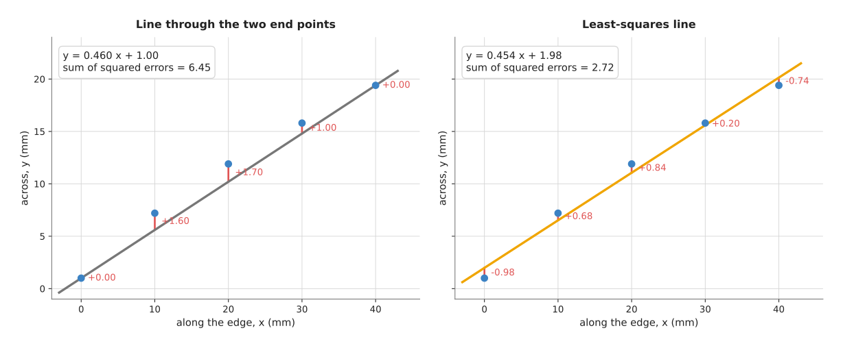
The line through the two end points has zero error at those two points, but large errors at the three in between, which add up to 6.45. The least-squares line instead misses every point by a little, and it adds up to 2.72. That is the smallest total any straight line can reach for these points.
A worked example: a line through five points#
That total of 2.72 is worth working out by hand, because doing the arithmetic once shows where such a number comes from. The table below lists the same five points from the picture, in millimetres.
| x | 0 | 10 | 20 | 30 | 40 |
|---|---|---|---|---|---|
| y | 1.0 | 7.2 | 11.9 | 15.8 | 19.4 |
Think of every possible line as one point on a map, with the slope m on one
axis and the offset c on the other. Then give each point on that map the sum
of squared errors of its line. The result is a bowl, because the total error is
high at the edges of the map and lowest near the middle. The picture below draws
that bowl as contour lines, like the height lines on a hiking map.
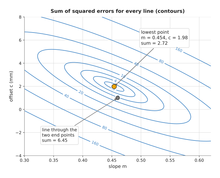
Each ring joins lines with the same total error. The orange dot at the centre is the least-squares line. The grey dot is the line through the two end points, which sits outside the ring marked 6, since its own total is 6.45.
At the bottom of a bowl the ground is flat in every direction. So the best line
is the one where a small change to m does not change the total. The same has
to be true of a small change to c. Writing those two conditions out gives two
ordinary equations, called the normal equations, which for a line are these:
(sum of x·x) · m  +  (sum of x) · c  =  sum of x·y
(sum of x)   · m  +  (number of points) · c  =  sum of y
Putting the five measured points into those sums gives the numbers below.
- sum of x·x = 0 + 100 + 400 + 900 + 1600 = 3000
- sum of x = 100
- sum of x·y = 0 + 72 + 238 + 474 + 776 = 1560
- sum of y = 55.3
- number of points = 5
So for these five points the two normal equations become:
3000 m + 100 c = 1560
 100 m +   5 c = 55.3
Multiply the second by 20 and subtract it from the first: 1000 m = 454, so
m = 0.454. Then put that back into the second: 5 c = 55.3 − 45.4 = 9.9, so
c = 1.98. This is the best line: y = 0.454 x + 1.98.
The residuals of that line are −0.98, +0.68, +0.84, +0.20 and −0.74 mm, and their squares add up to 2.72. That is the number at the lowest point of the bowl above. The typical distance of a point from the line is called the root mean square (RMS) residual. It is the square root of 2.72 divided by 5, which comes to 0.74 mm. Because it is one number in millimetres, the RMS residual is a useful summary of how well a fit went, and the rest of this page leans on it.
Because there is one normal equation per parameter, a shape with more parameters
works in exactly the same way. A computer then solves all of the equations at
once. In matrix form the equations are written AᵀA p = Aᵀb, where each row of
A holds one point's values. Then b holds the measured values and p holds
the parameters. You do not need to solve these by hand, since every numerical
library has a function for it.
The steps as pseudocode#
Since a library does the solving, it is worth seeing the order of the steps
first. The pseudocode below fits any shape whose error is a straight sum of
parameters times known values. That covers lines, planes written as
z = a x + b y + c, polynomials and the circle trick later on this page.
function fit_least_squares(points):
    A = empty table with one row per point
    b = empty list with one value per point
    for each point in points:
        add a row to A: the values that multiply each parameter
                        (for a line y = m x + c: [x, 1])
        add to b: the measured value (for a line: y)
    # the normal equations: (A-transpose times A) p = A-transpose times b
    p = solve (transpose(A) · A) p = transpose(A) · b
    residuals = b − A · p
    rms = square root of (sum of residuals squared / number of points)
    return p, rms
In practice a library solves the problem with a method called QR or the
singular value decomposition, instead of forming AᵀA directly. The answer is
the same either way, but those methods lose fewer decimal places when the
numbers are large or nearly repeat.
Planes: the singular value decomposition#
A table, a wall or the face of a box is a plane, so the pseudocode above looks
as though it already covers them. You could fit a plane as z = a x + b y + c,
with vertical residuals as for the line. That works well enough for a table seen
from above. However, it fails for a wall, because a wall is nearly vertical, and
a vertical plane cannot be written as "z equals something". The vertical gaps
also measure the wrong thing on a steep surface, so a plane needs its own
method.
Instead, the better way measures each point's distance at right angles to the plane. It uses a tool called the singular value decomposition (SVD), which in plain words does this:
- Take the average of all the points, which is the centre, and the plane passes through it.
- Subtract the centre from every point, so the points sit around the origin.
- The SVD finds the three directions in which the points spread out, one at right angles to the next, and how far they spread in each: the longest spread, the middle one and the thinnest one.
- For points on a flat surface the thinnest direction points straight out of the surface, and so it is the plane's normal, the direction the plane faces.
- The plane is "all points whose offset from the centre is at right angles to the normal".
The thinnest direction is exactly the one that makes the sum of squared right-angle distances smallest. So this is a least-squares fit too, even though no normal equations were written out. The picture below shows the result for 150 points on the tilted face of a board.
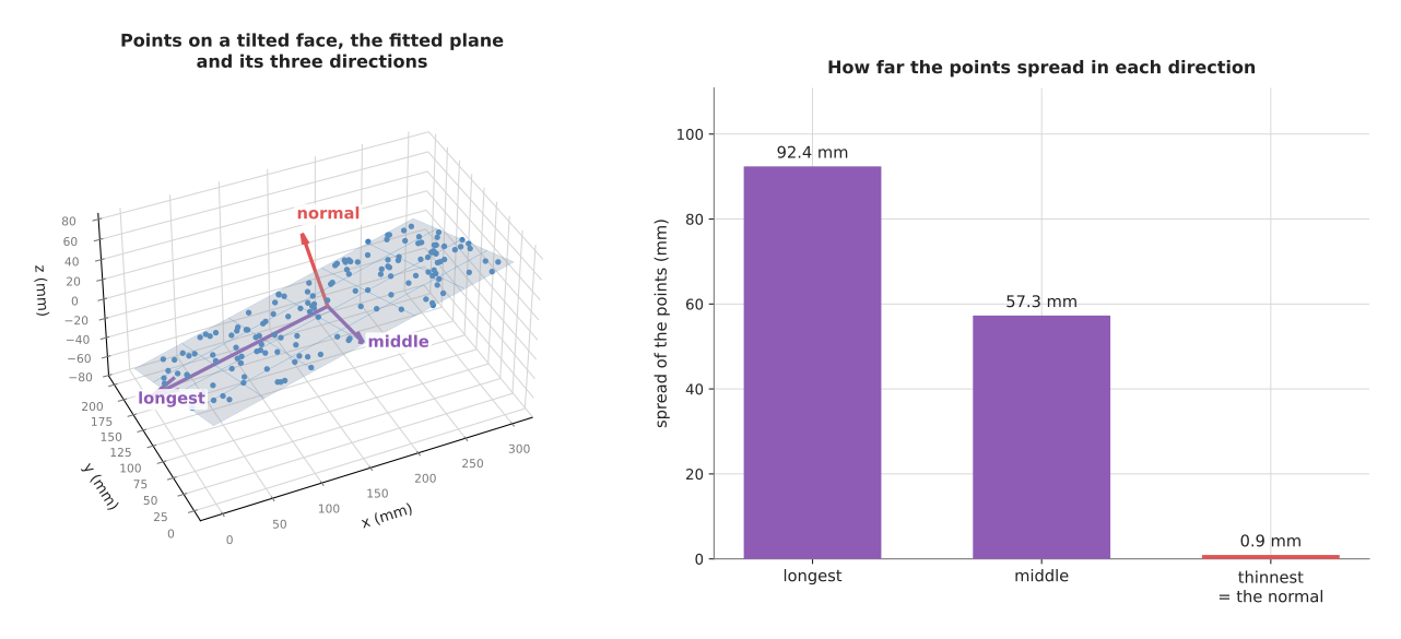
The points spread 92.4 mm along the longest direction and 57.3 mm along the middle one. Along the thinnest direction they spread only 0.93 mm, and that thinnest direction is the normal. The fitted normal is (−0.230, 0.321, 0.919), while the true face used to make the points has the normal (−0.230, 0.322, 0.919), so the fit agrees to three decimal places. The spread of 0.93 mm along the normal is also the RMS distance of the points from the plane: the noise that was added was 1 mm.
Because the three spreads come back as well, they carry a free check. If the thinnest spread is not much smaller than the middle one, then the points do not lie on a plane at all. They might lie on a curved surface, or across two surfaces, so a program should test the spreads before it trusts the normal.
The same three directions, computed for the points of one object, give its long axis and its thin axis. So that is how a program finds which way a box or a pen lies. The NumPy page in Book 1 shows this in which way an object lies.
Circles: a trick that keeps it simple#
Lines and planes both drop straight into the normal equations, but a circle does
not, so it needs one extra step first. Cups, glasses, bottle caps and holes are
all round objects. Seen from above, their rim is a circle with a centre (a, b)
and a radius r. The natural error is each point's distance from the circle,
but that error does not make a straight sum of parameters, so the normal
equations do not apply directly.
A short piece of algebra fixes this in one step. Because a point (x, y) on the
circle satisfies (x − a)² + (y − b)² = r², multiplying that out and moving the
terms around gives this:
x² + y² = 2a · x + 2b · y + k where k = r² − a² − b²
Now the unknowns a, b and k appear only multiplied by known values 2x,
2y and 1. So this is the same shape of problem as the line, with three
parameters instead of two. That means you can solve it with the pseudocode
above, and then recover the radius as r = square root of (k + a² + b²). This
is called the algebraic circle fit, or the Kåsa fit after the person who
described it.
The picture below shows why the fit matters on a real arm. A camera looking at a glass from the front sees only the near half of its rim.
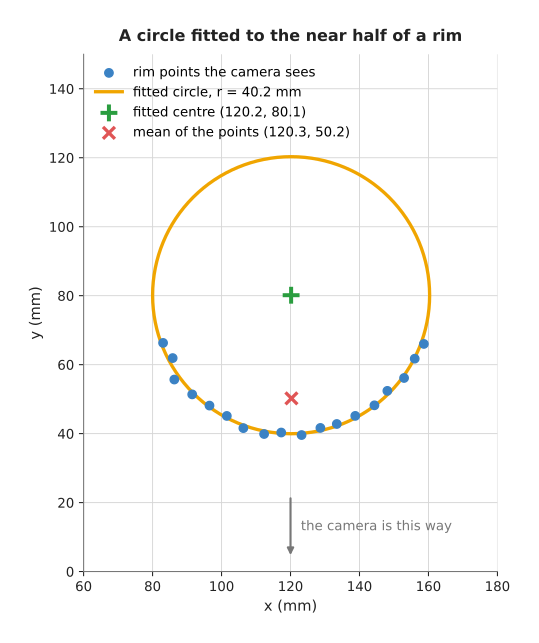
The 18 rim points came from a circle centred at (120, 80) mm with a radius of 40 mm, and they carry 0.6 mm of noise. The fit gives a centre of (120.2, 80.1) and a radius of 40.2 mm. The plain average of the points is (120.3, 50.2), and that lies 30 mm towards the camera, because all the points are on the near side. As a result, a gripper sent to the average would hit the front of the glass.
The algebraic fit does have one known weakness, which shows up when the points cover only a short arc. Below a quarter of the circle, it tends to give a radius that is too small. A second step, which minimises the true distances with a few rounds of nonlinear least squares, corrects this. The next section on the leftover error says how to spot the problem in the first place.
The leftover error tells you how good the fit is#
Every fit on this page returns an answer, and that is exactly where the danger lies. Least squares returns a line even for points that lie on a curve, and a plane even for points on two surfaces. That means the only sign that the shape is wrong is the leftover error.
So a careful program always returns the RMS residual with the fit, and compares it with the sensor's known noise. If a depth camera is good to about 1 mm and a plane fit leaves an RMS residual of 0.9 mm, then the plane is real. If it leaves 3 mm instead, then something else is in the points. That something might be an object on the table, the edge of the table, or a second surface. Book 2 makes the same point in report the margin, not the verdict.
4. Where it is used on a robot arm#
The sections above took lines, planes and circles one at a time. On a real arm those three fits turn up together, across perception, calibration, sensing and movement. The list below gives the most common places, and most of them link to a page that goes further.
- Finding the table's height and tilt. After RANSAC picks the points that belong to the table, an SVD plane fit on those points gives the most accurate plane. Every object's height is then measured from it.
- Measuring a round object. A program fits a circle to the rim of a cup or
glass, as above, to find where to aim the gripper. The glass-picking project
in the sibling repo does exactly this in
detect.py, with the samex² + y² = 2ax + 2by + ktrick. - Finding which way a face points. Before a wrist turns a board to lie flat, it must know the direction of the board's face. That is why the turn-top-flat project fits the face with the SVD, then refits with only the points within 6 mm, then 3 mm, then 2 mm, to drop the points from a neighbouring edge.
- Finding a straight edge in a picture. Edge pixels along a box side or a tray wall are fitted with a line, to give its angle for the gripper. The edges and contours page shows where these pixels come from.
- Correcting a sensor. Plot a distance sensor's readings against known true distances and fit a line, whose slope and offset then give the correction. Book 1 shows this in solving and fitting.
- Calibration. Camera calibration fits the camera's focal length and lens distortion to many checkerboard corners, while hand-eye calibration fits where the camera sits on the arm from many arm poses. Both are least-squares problems, and the calibration page explains them.
- Aligning two point clouds. Each step of iterative closest point finds the rotation and shift that best line up matched pairs of points, in the least-squares sense, using the SVD.
- Moving the arm to a pose. Numerical inverse kinematics repeatedly solves a small least-squares problem for how much to turn each joint. The page on numerical inverse kinematics calls this damped least squares.
- Learning a contact constant. A robot that pushes objects can fit the friction of the table from many pushes, one equation per push. The contact-parameters page in the sibling repo does this, and moves on to recursive least squares, which updates the fit one push at a time.
5. Where it is useful, and where it is not#
Those uses all assume the fit can be trusted, so this section says when it can be. Least squares is the right choice when every point belongs to the shape, the noise is small and spread evenly, and you know the shape in advance. In that case it is exact, fast and needs no settings.
Because the errors are squared, its big weakness is stray points: one point far from the rest pulls the answer hard. In the worked example above, change the last point from 19.4 to 29.4, as a depth camera might report for a single bad pixel. Then the fitted slope jumps from 0.454 to 0.654, and the offset from 1.98 to −0.02. That means one bad point out of five has moved the whole line.
The table below lists the common ways least squares goes wrong, and each of them has a standard cure. Read each row as a cause, the sign you would see, and what people use instead.
| What goes wrong | The sign you would see | What to use instead |
|---|---|---|
| Some points belong to something else (an object on the table, a stray reading) | RMS residual much larger than the sensor's noise; the shape is tilted towards the stray points | RANSAC to pick the good points first, or a robust loss that counts large errors less |
| Two surfaces in the same points | the thinnest SVD spread is not much smaller than the middle one | split the points first with clustering or RANSAC |
| The shape is wrong (a curve fitted with a line, an oval with a circle) | the residuals are not random: they are positive in the middle and negative at the ends | fit the right shape, or a polynomial of higher degree |
| A circle fit to a short arc | the radius comes out too small; the centre moves a lot when one point changes | a geometric fit with nonlinear least squares, or a known radius |
| Points cover a very small area | two parameters trade against each other; the fit changes a lot with the noise | measure over a wider area, or fix one parameter from other knowledge |
| Some points are more accurate than others (a depth camera is worse far away) | residuals are larger at one end | weighted least squares, which gives each point a weight |
| The errors are not a straight sum of parameters (distances to a circle, a camera's projection) | the simple solve gives a biased answer | nonlinear least squares, such as the Gauss-Newton or Levenberg-Marquardt method, which repeat a linear fit and improve the guess each time |
6. Libraries that provide it#
Since the cures in that table are all standard, you rarely write the solve yourself. The table below lists the well-known libraries that do it for you. Each row gives the library, the languages it is used from, the function or class and a note.
| Library | Languages | Function or class | Note |
|---|---|---|---|
| NumPy | Python | numpy.linalg.lstsq, numpy.polyfit, numpy.linalg.svd | the first thing to reach for; svd for planes |
| SciPy | Python | scipy.optimize.least_squares, scipy.optimize.curve_fit | nonlinear least squares, with robust losses such as soft_l1 and huber |
| OpenCV | C++, Python | cv::fitLine, cv::fitEllipse, cv::solve | line and ellipse fits on image points; fitLine also has robust distance options |
| Eigen | C++ | JacobiSVD, BDCSVD, ColPivHouseholderQR | the matrix library under most C++ robotics code |
| Open3D | Python, C++ | PointCloud.estimate_normals | fits a small plane around every point to get its normal |
| PCL (Point Cloud Library) | C++ | pcl::NormalEstimation, pcl::SACSegmentation | normals by local plane fit; model fitting with a least-squares refinement |
| Ceres Solver | C++ | ceres::Problem, ceres::Solve | large nonlinear least-squares problems, such as calibration |
| scikit-learn | Python | sklearn.linear_model.LinearRegression | the same line and plane fit, with a machine-learning style interface |
A plane fit with NumPy is three lines, since you subtract the mean, call svd
and take the last row of the result as the normal. Even the circle trick is only
one call to lstsq.
7. Why least squares, and what it costs#
Those libraries make the method easy to run, so it is worth saying plainly what it is and what it costs. Least squares is a way to choose a shape's parameters so that the sum of the squared distances from the points to the shape is as small as possible. In other words, it gives the arm clean numbers, such as a table height, a cup centre or an edge angle, from noisy points. It also gives a measure of how well the shape fits.
The obvious alternative is to use only a few special points. You could take the two end points of an edge, the highest and lowest points of a surface, or the middle of a bounding box around a rim. That takes no maths at all, but it throws away most of the data, and it lets the noise on those few points decide the answer. The worked example shows the difference, because the end-point line has more than twice the total error of the least-squares line. The glass example shows a worse case, since the average of the points is 30 mm off while the fit is 0.2 mm off. Least squares instead uses every point, so the noise averages out.
The second alternative is to minimise something other than squared distances, for example the plain sum of distances. That resists stray points better, but it has no direct solution. Instead it needs repeated steps, which are slower and can stop at the wrong answer. That is why squared distances are chosen: they give a direct, exact solution in one step.
Three costs come with that choice, and the first is that you must know which shape to fit before you start. Second, every point must belong to that shape, because one stray point can move the answer a long way. Third, the answer always looks confident, so you must check the leftover error yourself. That is why, when stray points are likely, you add RANSAC in front of the fit.
8. The learned alternative#
That comparison was with hand-picked points, so the other one a reader will want is with machine learning. Fitting a known shape, such as a table plane or a cup's rim, has no learned replacement. The shape's formula is known, and least squares gives its best fit exactly, in one step. So learning takes over only when nobody knows the shape in advance. Book 7's linear regression page shows that linear regression is least squares itself. Its Gaussian processes page shows that a Gaussian process, a method that gives an error bar with each prediction, can learn a curve that nobody wrote down, such as a depth camera's error against distance. A small neural network can learn the same kind of curve. However, with a few input numbers and tens to hundreds of examples, the classical methods do as well as the network or better. A network pulls ahead only when the input is a picture, a point cloud or a long recording, and there are many examples.
9. Where to read next#
- The next page is RANSAC, which finds which points belong to the shape, so that least squares can then fit only those.
- The Kalman filter applies the same idea to readings that arrive one at a time, rather than all at once.
- Iterative closest point uses an SVD least-squares fit inside each step to line up two point clouds.
- Numerical inverse kinematics uses damped least squares to move the arm to a pose.
- How a model learns in Book 6 shows that training a network is the same idea, because it makes the total error as small as possible, over millions of parameters instead of three.
- Book 2's methods you write yourself shows how a fitted table plane is used to measure objects standing on it.
10. Using it in Python#
Sections 3 and 6 established two things: that a least-squares fit comes down to solving one linear system, and that NumPy already has the routine that solves it. This section closes the gap between those two facts by showing the call itself. After it you will be able to fit a line and a plane to your own points, and you will know which of the numbers in the result you are allowed to trust.
The program below does both fits. The line fit uses numpy.linalg.lstsq, which
takes the matrix of rows described in section 3 and the measured values, and
returns the parameters that make the sum of the squared misses smallest. The
plane fit uses numpy.linalg.svd, because as section 3 explained a plane is
found by subtracting the mean from the points and taking the direction they vary
in least.
import numpy as np

# --- a line through five measured heights, in millimetres
x = np.array([0.0, 10.0, 20.0, 30.0, 40.0])
y = np.array([2.1, 4.2, 5.8, 8.3, 9.9])
A = np.column_stack([x, np.ones_like(x)])          # one row per point
(slope, offset), residuals, rank, singular = np.linalg.lstsq(A, y, rcond=None)
rms = np.sqrt(residuals[0] / x.size)               # the leftover error

# --- a plane through a patch of table points, in metres
points = np.loadtxt("table_patch.txt")             # N rows of x, y, z
centre = points.mean(axis=0)
u, s, vt = np.linalg.svd(points - centre)
normal = vt[-1]                                    # the direction the plane faces
thickness = np.sqrt(np.mean(((points - centre) @ normal) ** 2))
On the five heights above, that gives a slope of 0.197 and an offset of 2.12, with a leftover error of 0.18 mm. On 500 points scattered by 2 mm about a level table 0.72 m below the camera, the plane fit returns a normal of about (0.0003, 0.0005, −1.0) and a thickness of 2.1 mm, which recovers the scatter the points were given.
The libraries do the solve and nothing else. lstsq factorises the matrix and
returns the parameters, and it also hands back the sum of the squared misses in
residuals, the rank of the matrix and its singular values. Those three
extra outputs are the ones worth reading, because a rank lower than the number
of unknowns means the data does not pin all of them down, and a large spread
between the first and last singular value means the answer is fragile.
What you have to write is the matrix A, and that is the real work. Each column
of A says how one unknown enters the model, so writing A is the same as
writing down the model. The circle trick in section 3 is exactly this: it is a
rearranged A that turns a curved fit into a call to the same routine. You also
have to write the check afterwards, because lstsq always returns numbers and
never refuses.
What you have to decide or measure is what counts as a good fit. The rms above
is 0.18 mm, but only you know whether 0.18 mm is fine for the job the arm is
about to do, and only you know the sensor's own noise to compare it against. If
the leftover error is far larger than the sensor's noise, then either the shape
is wrong or some of the points do not belong to it, and the second of those is
what the RANSAC page solves. You also have to decide the units,
because the plane fit above is in metres while the line fit is in millimetres,
and lstsq will not notice if you mix them.