This page explains how a program finds the same small spots in two pictures, and how it uses those spots to say where a known flat object is. It does that by answering five questions, in the order in which a program answers them. Which spots in a picture are easy to find again? Then how does a program describe one of those spots as a list of numbers? How does it pair each spot in one picture with the right spot in the other? Once it has those pairs, how does it throw away the ones that are wrong? And what can a robot arm do with the pairs that are left?
It is for a reader who knows what a pixel and a grey picture are, and who has read nearest-neighbour search. That page matters here because pairing spots is itself a nearest-neighbour search, carried out on descriptions instead of positions. This page also uses RANSAC, a method that fits a model when some of the data is wrong. So it explains, as it goes, what it needs from both of those pages.
The work is usually called feature matching, and the word feature needs a clear meaning before anything else. So, on this page, a feature is a small spot in a picture that can be found again. It also carries a list of numbers that describes what the picture looks like around it.
Contents#
- The idea in one sentence
- How it works, step by step · The example: a printed label in a cluttered picture · Step one: find spots that are easy to find again · Step two: describe each spot · Step three: match the descriptions · Step four: the ratio test · Step five: clean up with RANSAC · The pseudocode
- Where it is used on a robot arm
- Where it is useful, and where it is not
- Libraries that provide it
- Why feature matching, and what it costs
- The learned alternative
- Where to read next
- Using it in Python
1. The idea in one sentence#
Feature matching picks out corners in two pictures, describes the little patch round each corner as a list of numbers, pairs each corner with the corner whose list is most alike, and keeps only the pairs that agree on one single movement of the object.
For example, imagine that you have a photo of a cereal box, and that you want to find that box on a crowded shop shelf. You do not compare the whole photo with the whole shelf. Instead you pick out a few distinctive bits of the box, such as the corner of a letter or the tip of a leaf in the logo. Then you look for those same bits on the shelf, and you ignore the bits that look alike on several boxes. Once several of the bits you found sit in the same arrangement as on the photo, you have found the box. That is why feature matching does the same work, in the same order.
2. How it works, step by step#
2.1 The example: a printed label in a cluttered picture#
The example used all the way through this page is a flat printed label, such as the label on a box of parts. The program has a stored picture of that label, 200 by 140 pixels. Then the camera takes a picture of a cluttered table, 320 by 230 pixels. Because the camera looks at the table from an angle, the label appears in that second picture turned by about 11°, a little smaller, and tilted. There is also a second, smaller sticker in the corner of the picture, and it carries part of the same print. That sticker is a trap, because its spots look exactly like spots on the label although it is not the label.
So the program's job is to find the label in spite of the sticker, and to say exactly where the label's four corners are in the camera picture.
All the numbers on this page come from the diagram script
docs/diagrams/searching_and_matching_2.py, which runs every step described
here. As a result, you can check any of them yourself by running it with
--numbers, which prints them.
2.2 Step one: find spots that are easy to find again#
The program cannot use every spot of that label, because not every spot in a picture can be found again. To see which spots can, think of a small square window placed on the picture. Then shift that window by a pixel or two, and ask how much the picture inside it changes. The picture below does this for three windows, one on a flat area, one on an edge and one on a corner.
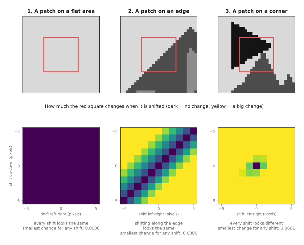
The top row shows the three windows as red squares. The bottom row then shows how much each window's contents change for every shift up to 5 pixels in each direction. Dark there means no change, while yellow means a big change.
- On a flat area, nothing changes whichever way the window moves, so the smallest change for any shift is 0.0000 and a spot there could be anywhere in the flat area.
- On an edge, the window changes when it moves across the edge but not when it slides along it, so the smallest change is again 0.0000 and a spot there could be anywhere along the edge. The dark stripe in the middle panel is the direction of the edge.
- On a corner, every shift changes the window, so the smallest change for any shift is 0.0601 and a corner can be found again to within a pixel.
That is why a program looks for corners, and the best-known test for them is the Harris corner detector. It measures, at every pixel, how much the brightness changes in the direction where it changes most, and in the direction where it changes least. Then it calls a pixel a corner when even the smaller of those two changes is large. The program also keeps only the pixel with the highest score in each small neighbourhood, so that one corner does not give ten spots.
In the example this finds 46 corners in the stored label and 161 in the camera picture. The camera picture has more because it also shows the clutter round the label.
The word keypoint is often used for a spot found this way. Instead of corners, some other detectors look for blobs, which are small round patches that are darker or brighter than their surroundings. The idea behind both is the same, because a good keypoint is one that moves with the object and nowhere else.
2.3 Step two: describe each spot#
Because step one gives nothing but positions, the program cannot yet tell one keypoint from another. To pair a keypoint with a keypoint in the other picture, it also needs to know what the picture looks like round that spot. So it turns the patch round each keypoint into a list of numbers, called a descriptor. Two patches that look alike then get lists that are alike, which is what makes pairing possible at all.
The example uses the idea inside ORB, which is the most common fast descriptor, and it works in the four steps below.
- Smooth the picture a little, so that single noisy pixels matter less.
- Find the patch's own direction. The program takes the "centre of brightness" of the round patch and draws an arrow from the keypoint to it, and if the object turns, this arrow turns with it.
- Compare pairs of pixels. The program has a fixed list of 256 pairs of positions inside the circle, and it turns that whole list to the patch's own direction, so that for each pair it can ask one question: is the first pixel darker than the second? The answer is 1 for yes and 0 for no.
- The 256 answers, in order, are the descriptor: a string of 256 bits.
The picture below shows what those four steps give for one keypoint of the label, next to two keypoints from the camera picture.
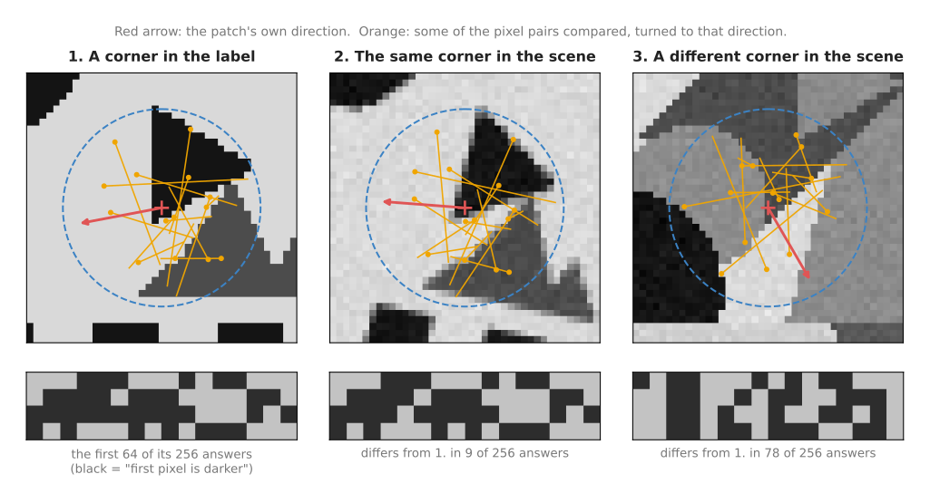
The first panel is a corner in the stored label. The second panel is that same corner in the camera picture, where the label has been turned. Its arrow therefore points 15° further round, and the pixel pairs turn with the arrow, so they land on the same parts of the pattern. As a result the answers differ in only 9 of the 256 bits. The third panel is some other corner in the camera picture, and its answers differ in 78 of the 256 bits.
The number of bits that differ between two descriptors is called the Hamming distance. Because a computer can count differing bits very fast, it is the distance that this kind of descriptor uses.
Three descriptors are worth knowing by name, and they all do the job described above in different ways. So read the table below one row at a time, as one descriptor, what it stores, and how two of its lists are compared.
| Descriptor | What it stores | How two are compared | In plain words |
|---|---|---|---|
| ORB (Oriented FAST and Rotated BRIEF, 2011) | 256 bits | Hamming distance | fast; handles turning; handles size change by searching a stack of smaller copies of the picture |
| SIFT (Scale-Invariant Feature Transform, 1999 and 2004) | 128 numbers | ordinary straight-line distance | counts the directions of brightness change in a 4 by 4 grid of small squares round the keypoint; slower, but handles size change, turning and light changes very well |
| AKAZE (Accelerated KAZE, 2013) | a few hundred bits | Hamming distance | finds keypoints in a way that keeps object edges sharp; between ORB and SIFT in speed and quality |
In that table, "handles size change" means that the same patch seen from closer or further away still gets a similar descriptor. However, the example on this page only uses one picture size, because the label is only a little smaller in the camera picture than in the stored one.
2.4 Step three: match the descriptions#
Once every keypoint carries a descriptor, the program can pair the keypoints up. For each keypoint in the label, it finds the keypoint in the camera picture whose descriptor is closest. This is a nearest-neighbour search, but in the space of descriptors rather than in the space of positions. With a few hundred keypoints the program simply measures every pair, while with tens of thousands it uses an approximate search instead.
In the example, 38 of the 46 label keypoints get a right partner. A pair counts as right when the partner lies within 3 pixels of where the label corner really is. Because the diagram script made the camera picture itself, it knows where every label corner really is. That is why the other 8 pairs are known to be wrong, although a real program would not know which ones.
2.5 Step four: the ratio test#
However, some wrong pairs can be spotted even without knowing which ones are wrong. If a keypoint's best partner is only a little better than its second-best partner, the program cannot really tell the two apart. This happens on repeated patterns, such as the row of identical squares along the bottom of the label.
The ratio test, from David Lowe's 2004 SIFT paper, uses exactly that difference, because it keeps a pair only when
distance to the best partner < 0.8 × distance to the second-best partner
The number 0.8 in that rule is the one Lowe suggested. The picture below then shows what the test does to every label keypoint.
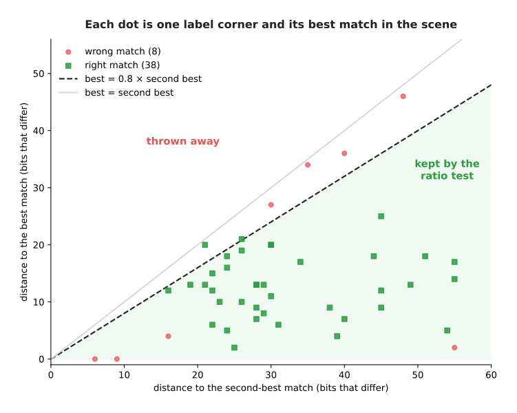
Each dot in it is one label keypoint, placed to the right by the distance to its second-best partner and up by the distance to its best partner. So the dots below the dashed line are the ones that pass the test. For example, the corner-shaped patch from step two has a best partner that differs in 9 bits and a second-best that differs in 28. Its ratio is therefore 0.32, and the pair is kept.
The table below counts what happened to all 46 pairs. So read each row as one kind of pair, and the two columns as what the ratio test did with pairs of that kind.
| Pair | Kept | Thrown away |
|---|---|---|
| right | 36 | 2 |
| wrong | 4 | 4 |
The ratio test threw away half of the wrong pairs and lost only 2 right ones. But 4 wrong pairs passed it easily, and they are the dots in the bottom left corner of the picture. Because all four of them point at the second sticker, two of them even have a distance of 0. That sticker carries the same print, so these pairs look perfect on their own. In other words, no test that looks at one pair at a time can catch them.
2.6 Step five: clean up with RANSAC#
Since no test on a single pair can catch those last four, the final step uses a fact about the pairs as a group. The right pairs agree with each other, while the wrong ones do not. The label in this example is flat, and that is what lets them agree. When a flat object is seen by a camera, every point on it moves from the stored picture to the camera picture by one and the same rule, which is called a homography. A homography is a 3 × 3 table of numbers that maps the points of one flat surface to the points of another. It also includes the effect of looking at that surface from an angle, and it can be computed from four pairs of points. Calibration uses the same kind of mapping for its flat checkerboard.
Because the wrong pairs do not agree with the homography of the right pairs, the program uses RANSAC. That name stands for random sample consensus, and the method repeats the four steps below many times over.
- Pick four pairs at random.
- Compute the homography that fits those four exactly.
- Move every label keypoint by that homography, and count how many of them land within 3 pixels of their partner, because those pairs are the inliers.
- Remember the homography with the most inliers.
At the end it computes the homography again from all the inliers of the best try. The picture below then shows the result on the example.
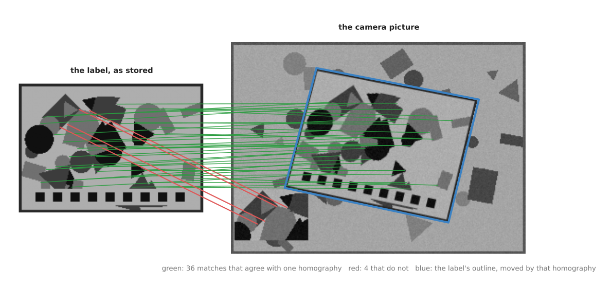
Of the 40 pairs left after the ratio test, 36 agree with one homography, and RANSAC found it on its 18th try. As a result, the 4 red pairs, which point at the second sticker, are thrown away. The blue outline is the label's edge, moved by the final homography. Each of its four corners is within 0.75 pixels of where the label corner really is.
With 36 inliers out of 40, nine pairs in ten are right, and the RANSAC page gives the rule for how many tries are enough. For four pairs at a time and nine in ten right, 5 tries already give a 99% chance of one clean try. So the 1,000 tries the script ran are far more than needed, and real programs stop early once they find a good answer.
2.7 The pseudocode#
All five steps together fit in the pseudocode below, which is written in plain steps rather than in any real programming language.
find_flat_object(stored_picture, camera_picture):
    # step one and two: keypoints and descriptors, in both pictures
    keys_a, desc_a = detect_and_describe(stored_picture)
    keys_b, desc_b = detect_and_describe(camera_picture)

    # step three and four: match, then the ratio test
    pairs = empty list
    for each i in keys_a:
        best, second = the two descriptors in desc_b closest to desc_a[i]
        if distance(desc_a[i], best) < 0.8 * distance(desc_a[i], second):
            add (keys_a[i], position of best) to pairs
    if number of pairs < 4: return "not found"

    # step five: RANSAC
    best_inliers = empty
    repeat many times:
        four = 4 pairs chosen at random from pairs
        H = homography that maps the four exactly
        inliers = pairs where distance(H applied to a, b) < 3 pixels
        if inliers has more pairs than best_inliers:
            best_inliers = inliers
    if number of best_inliers < a minimum, such as 10: return "not found"
    H = homography fitted to all of best_inliers
    return H

detect_and_describe(picture):
    score = corner score of every pixel              # Harris, or FAST
    keys = pixels whose score is the highest in their neighbourhood
    for each key in keys:
        direction = direction from key to the centre of brightness of its patch
        desc[key] = for each of the 256 pixel pairs, turned to direction:
                        1 if first pixel is darker than second, else 0
    return keys, desc
The minimum number of inliers in that code matters more than it looks. Because RANSAC always returns its best try, it returns one even when the object is not in the picture at all. A few random pairs can agree with each other by chance. That is why a rule such as "at least 10 inliers" turns that best try into a clear "not found".
3. Where it is used on a robot arm#
All five steps together answer one question for an arm, which is where a known object is. So feature matching is used wherever the arm has to find an object that has printing or texture on it, from a camera picture alone.
- Finding a textured part or package. A box of screws, a bag of coffee or a book has printing on it, so the program stores one picture of each face. Feature matching then finds that face in the camera picture, even when it is turned, partly hidden by other objects, or seen from an angle.
- The pose of a flat object from a homography. When the object is flat, or has a flat face, the homography says where every point of that face is in the picture. With the camera's lens numbers from the pinhole camera model, the homography can be turned into the face's position and turn in 3D. As a result, it works for a sheet of paper, a label, a circuit board or the lid of a box.
- Feeding pose from points. When the object is not flat, the program stores a 3D model whose surface points each carry a descriptor, and feature matching pairs those points with keypoints in the camera picture. Those 3D-to-2D pairs are exactly what pose from points (the perspective-n-point problem, or PnP) needs to compute the object's 3D pose, and RANSAC is again used to throw away wrong pairs.
- A first guess for ICP. A pose from feature matching is often a few millimetres off. Iterative closest point on a depth scan can finish it off, because the feature pose is a good first guess.
- Following the camera's own movement. A camera on the wrist sees the table from a slightly different place in each picture, so matching keypoints from one picture to the next says how the camera moved. This is the core of visual odometry, and of the wider method in multi-view geometry.
- Keeping track of objects. Book 2's tracking and association uses keypoint descriptors such as ORB to tell apart two objects that sit close together, when position alone cannot.
4. Where it is useful, and where it is not#
All of those uses assume that the object gives the program something to match. Feature matching is reliable on objects with plenty of printing or texture, seen from roughly the angles in the stored picture. But it fails when there is nothing to find, or when there is too much that looks the same.
The table below lists the common problems that follow from that. So read each row as one thing that goes wrong, the sign you see when it does, and what people use instead.
| Problem | The sign you see | What people use instead |
|---|---|---|
| The object has no texture, such as plain grey plastic or a painted metal part | only a handful of keypoints on the object, and RANSAC finds too few inliers | a depth scan and ICP, the object's outline from edges and contours, or a learned pose model |
| A shiny surface | keypoints on reflections, which move when the camera moves, so the inliers change from frame to frame | light from another angle, a polarising filter, or a depth camera |
| A repeated pattern, such as a grid, a barcode or woven fabric | the ratio test throws away most pairs | match on the parts of the object that do not repeat; add a printed marker |
| Two copies of the same object, or of the same print | RANSAC locks onto one copy, and may switch between them from frame to frame | find one copy, remove its inliers, and run RANSAC again to find the next |
| A large change in viewing angle, more than roughly 40° to 60° of tilt from the stored picture | few pairs pass the ratio test, although the object is in plain sight | store pictures of the object from several angles, or use a learned matcher |
| Motion blur, from a moving arm or camera | corners smear out and are not found | take the picture when the arm is still; shorten the camera's exposure time |
| The object is not flat, but a homography is fitted | RANSAC finds only the inliers on one face | fit a pose with PnP from a 3D model instead of a homography |
When nothing on the object itself can be relied on, people often stick a printed marker on it, such as an ArUco or AprilTag marker. Such a marker is a black and white square, designed to be found and identified without any matching step at all.
5. Libraries that provide it#
None of those five steps has to be written from scratch, and the table below lists the well-known libraries that already provide them. In it, the "functions or classes" column gives the names to look up in each library's own documentation.
| Library | Languages | Functions or classes | Note |
|---|---|---|---|
| OpenCV | C++, Python | cv2.ORB_create, cv2.SIFT_create, cv2.AKAZE_create; cv2.BFMatcher and its knnMatch for the two nearest partners; cv2.findHomography with cv2.RANSAC; cv2.solvePnPRansac | the usual choice; SIFT has been in the main package since version 4.4, after its patent ran out in 2020 |
| scikit-image | Python | skimage.feature.corner_harris, skimage.feature.ORB, skimage.feature.SIFT, skimage.feature.match_descriptors (its max_ratio argument is the ratio test), skimage.measure.ransac | easy to read and step through; slower than OpenCV |
| Kornia | Python (PyTorch) | kornia.feature.LoFTR, kornia.feature.LightGlue | learned matchers, run on a graphics processor |
| LightGlue | Python (PyTorch) | the lightglue package, with SuperPoint and LightGlue classes | the authors' own code for SuperPoint plus LightGlue |
For a first try on a robot arm, OpenCV's ORB with a brute-force Hamming matcher,
the ratio test and cv2.findHomography is a few lines of code and runs on an
ordinary processor.
6. Why feature matching, and what it costs#
Now that the steps and the libraries are covered, this section answers the four questions that decide whether to use the technique at all. Those questions are what it is, what it does for you, why it rather than the obvious alternative, and what it costs.
Feature matching finds small distinctive spots in two pictures, describes them as lists of numbers, pairs them, and keeps the pairs that agree on one movement. So it tells you where a known textured object is in a picture, and, with a flat face or a 3D model, where that object is in 3D. It needs no training data at all, because one picture of the object is enough.
The obvious alternative is template matching, which slides the whole stored picture over the camera picture, pixel by pixel. Then it keeps the place where the two look most alike. It is simple, and it works well when the object is always the same way up and the same size. For example, a part sitting in a fixed tray is always the same way up and the same size. But it fails as soon as the object is turned, tilted, nearer or further away, or partly covered. Each of those needs its own set of slides, and a partly covered object never looks like the stored picture. Because it only needs some of the spots to be visible, feature matching handles all of them, and each spot is also described in a way that survives turning.
Those advantages come with costs that show up in every real program. The object must have texture or printing on it, and wrong pairs are normal, so RANSAC and a minimum inlier count are always needed. Then the thresholds, such as the ratio 0.8, the 3-pixel limit and the minimum number of inliers, need tuning for each camera and object. And the result is only a pose in the picture. So to get a pose in the arm's frame, you also need the camera's lens numbers and its calibration to the arm.
7. The learned alternative#
Since about 2018, neural networks have been trained to do steps one to four in place of the classical methods above. SuperPoint, for example, finds and describes keypoints in one single network. Then SuperGlue and the later LightGlue, from 2023, pair the keypoints of two pictures by looking at all of them together. LoFTR goes further and skips keypoints, matching the two pictures directly. They find many more right pairs on hard pictures, such as large changes of angle, poor light and little texture. Even so, RANSAC is still used after them in the same way. But they need a graphics processor to run at camera rate and a large set of model weights, and it is harder to see what went wrong when they fail. Book 7's keypoints and object pose describes networks that find an object's named points and its pose directly, and tracking and motion describes point trackers that follow spots from picture to picture. So a classical matcher is still the better first choice when the object has good texture and the camera angle does not change much, because it needs no training and one stored picture is enough.
8. Where to read next#
- RANSAC explains the clean-up step in more depth, including how many tries are enough.
- Pose from points turns matched 3D model points and picture points into a 3D pose.
- Multi-view geometry uses matched keypoints from two pictures to work out how the camera moved and how far away things are.
- Iterative closest point does the same job on depth scans, and its section on getting a first guess uses 3D features in the same way that this page uses picture features.
- The chapter overview shows how this page fits with the others.
9. Using it in Python#
Section 2 took the five steps in order, from finding corners to keeping only the pairs that agree on one movement, and section 5 named the OpenCV calls for each step. This section puts them together, because the whole of section 2 is about fifteen lines of Python and seeing them in one place makes the division of labour clear. After reading it you should be able to find a known flat object, such as a printed label, in a camera picture.
The example uses ORB, which is the detector and descriptor combination section 5 recommends for a first try on an arm, because it runs fast on an ordinary processor and needs no graphics card.
import cv2
import numpy as np

stored = cv2.imread("label.png", cv2.IMREAD_GRAYSCALE)   # the object, photographed once
live = cv2.imread("shelf.png", cv2.IMREAD_GRAYSCALE)        # what the camera sees now

orb = cv2.ORB_create(nfeatures=1000)
keypoints1, descriptors1 = orb.detectAndCompute(stored, None)
keypoints2, descriptors2 = orb.detectAndCompute(live, None)

# Pair each spot with its two most similar spots. Hamming distance counts the bits
# that differ, which is the right measure for ORB's descriptions.
matcher = cv2.BFMatcher(cv2.NORM_HAMMING)
pairs = matcher.knnMatch(descriptors1, descriptors2, k=2)

# The ratio test: keep a pair only when the best partner is clearly better than the
# second best, because an ambiguous pair is usually a wrong one.
good = [best for best, second in pairs if best.distance < 0.75 * second.distance]

source = np.float32([keypoints1[m.queryIdx].pt for m in good]).reshape(-1, 1, 2)
target = np.float32([keypoints2[m.trainIdx].pt for m in good]).reshape(-1, 1, 2)

H, mask = cv2.findHomography(source, target, cv2.RANSAC, ransacReprojThreshold=3.0)
print(int(mask.sum()), "of", len(good), "pairs agree on one movement")
What the library does for you is all five steps. detectAndCompute finds the
corners and describes the patch round each one in a single call, knnMatch runs the
nearest-neighbour search over the descriptions, and findHomography with
cv2.RANSAC fits the one movement that most pairs agree on while ignoring the rest.
Each of those would be a long piece of code to write, and none of them is worth
writing.
What you still write yourself is the ratio test and the verdict. The ratio test is
that one list comprehension, and OpenCV does not do it for you, which is why every
tutorial contains the same line. You also decide what counts as having found the
object, because findHomography returns a matrix whenever it has four pairs to work
with, and a matrix fitted to four wrong pairs looks exactly like a matrix fitted to
four right ones. The usual test is to count the inliers in mask and require at
least ten or fifteen, and then to check that the four corners of the stored picture,
carried through H with cv2.perspectiveTransform, still make a sensible convex
shape rather than a bow tie.
What you have to decide or measure is three numbers. The nfeatures limit trades
time against the chance of finding the object, and 500 to 2,000 is the usual range.
The 0.75 in the ratio test is the standard value from the original paper, and
lowering it towards 0.6 throws away more pairs but leaves cleaner ones, which is
what you want on a repeated pattern. The ransacReprojThreshold is in pixels and
says how far a pair may sit from the fitted movement and still count, so 3 pixels is
a reasonable start and it should reflect how accurately your corners are located.
Finally, remember what section 4 says: none of these numbers helps on an object with
no texture, and no amount of tuning will find a plain white box this way.