This page explains iterative closest point (ICP): a method that moves one set of points onto another set of points that shows the same shape. On a robot arm, the first set is usually a stored model of a part, and the second is a depth scan of the real part. So ICP answers the question "exactly where is the part, and which way is it turned?". This page shows how ICP works, round by round, on a small example with real numbers. It then shows when ICP gives a wrong answer, and how you can tell that it has.
It is written for a reader who has already read nearest-neighbour search , because every round of ICP runs that search. It also helps to know what a rotation and a shift are, from rigid transforms , although this page explains each term where it needs it.
Contents#
- The idea in one sentence
- How it works, step by step · The example: a bracket on a table · Step one: pair each model point with its closest scan point · Step two: the best move for those pairs · Repeat until the gap stops shrinking · The pseudocode · Point-to-plane: a faster version
- Where it is used on a robot arm
- Where it is useful, and where it is not
- Getting a first guess: 3D features and global registration · Surface normals · Local 3D features · Matching features, then RANSAC · Finishing with ICP · Where it is used, where it fails, and libraries
- Libraries that provide it
- Why ICP, and what it costs
- The learned alternative
- Where to read next
- Using it in Python
1. The idea in one sentence#
ICP guesses which scan point each model point belongs to by taking the closest one, moves the model to fit those guesses as well as possible, and repeats until the model stops moving.
The move ICP finds is a rigid transform, which means a rotation plus a shift with no stretching and no bending. That is the right kind of answer, because a part lying on a table cannot change its shape.
Here is an everyday example of the same loop. Suppose you have a paper outline of a key, and you want to lay it over the real key lying on a table. You put the paper down roughly where the key is. Then you see that each edge of the paper sits a little to the left of the matching edge of the key. Because of that, you slide the paper to the right and turn it a little. Now the edges are closer, which means you can see better which edge of the paper goes with which edge of the key, so you slide and turn again. After a few small moves the paper sits on the key, and ICP does the same thing with points instead of edges.
2. How it works, step by step#
Section 1 described the loop in words, and this section walks through that same loop on one small example, one round at a time. So every claim made about it here comes with a number you can check.
2.1 The example: a bracket on a table#
The example is an L-shaped metal bracket lying flat on a table, seen from above by a depth camera. It is kept flat only so that the pictures fit on a page. A real scan has three coordinates per point, but every step below works the same way in 3D.
- The model is the bracket's outline as it was drawn: 120 mm long, 80 mm high, with arms 30 mm wide. It has one point every 10 mm round the outline, 40 points in all.
- The scan is what the camera saw, with one point every 6 mm and 66 points in all. Each point is moved by a small random amount, the way a real depth camera's points are. That random amount has a standard deviation of 0.8 mm in each direction, and the standard deviation is the typical size of a random error.
- The real bracket is turned 20° from the model and shifted by 30 mm in x and 20 mm in y, and ICP is not told any of this, because finding it is its job.
- ICP starts from a first guess: the model exactly where it was drawn, not turned and not shifted.
All the numbers on this page come from the diagram script
docs/diagrams/searching_and_matching.py, which runs exactly the ICP described
here. That is why you can run that script with --numbers and print the numbers
yourself.
2.2 Step one: pair each model point with its closest scan point#
Because ICP does not know which scan point belongs to which model point, it starts by guessing: each model point is paired with the scan point nearest to it. That guess is a nearest-neighbour search run once for every model point, and the pairs it produces are called correspondences.
The picture below shows the pairs that this first search produces, before the model has moved at all.
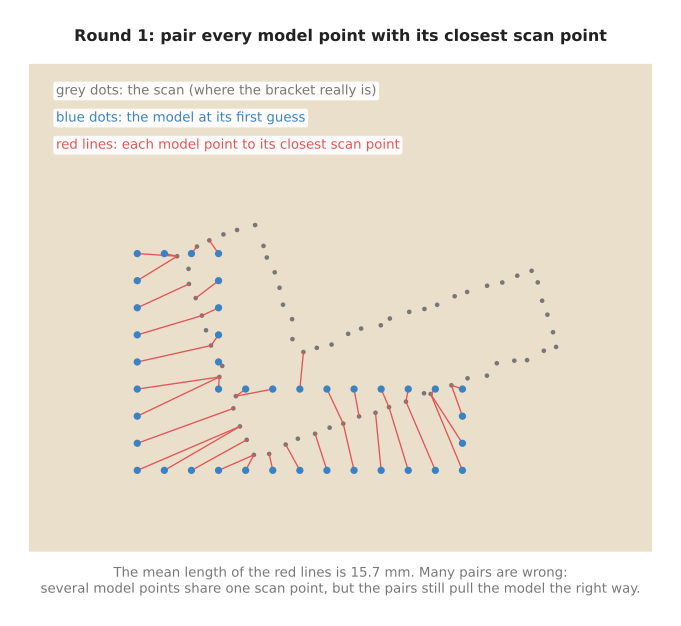
Many of these pairs are wrong, because the model points along the left edge all reach across to the scan's left edge, which is higher up and turned. Several model points even share one scan point. The mean length of the red lines, called the mean gap on this page, is 15.7 mm.
The pairs are wrong, but they are not random, because on the whole they pull the model up, to the right, and anticlockwise. That is already enough, since the next step only needs to move the model in roughly the right direction.
2.3 Step two: the best move for those pairs#
Once the pairs exist, ICP works out the one rotation and shift that brings each model point as close as possible to its partner. "As close as possible" means that the sum of the squared distances between partners is as small as it can be. There is an exact method that finds this move, and it takes three steps.
- Find the middle of the model points, and the middle of their partners. The middle is the average of all the x values and of all the y values. It is called the centroid.
- Measure every model point from the model's centroid, and every partner from the partners' centroid. Now both sets are centred on the same spot. Find the turn that lines the first set up with the second as well as it can. A standard piece of linear algebra, the singular value decomposition (SVD), gives this turn directly. The method is known as the Kabsch method, or the Umeyama method.
- The shift is whatever then moves the turned model's centroid onto the partners' centroid.
Here is the same method on three points, which is small enough to check by hand. The model is a triangle with corners (0, 0), (40, 0) and (0, 20). The partners are that same triangle turned 30° and shifted by (10, 5), so their corners are (10.00, 5.00), (44.64, 25.00) and (0.00, 22.32).
- The model's centroid is (13.33, 6.67). The partners' centroid is (18.21, 17.44).
- Centred on their centroids, the two triangles differ only by a turn. The SVD finds it: 30.0°.
- Turning the model's centroid by 30° about the origin moves it to (8.21, 12.44). The shift that takes it to (18.21, 17.44) is (10.00, 5.00).
The method finds the turn and the shift exactly, because in this small example the pairs are right. In ICP itself the pairs are only guesses, so the move the method finds is only partly right. The model is then moved by it, and ICP goes back to step one.
2.4 Repeat until the gap stops shrinking#
Because each move brings the model closer to the scan, the pairs found after it are better, which means the next move is better as well. The picture below shows the model at the start, after one round, after four rounds, and at the end.
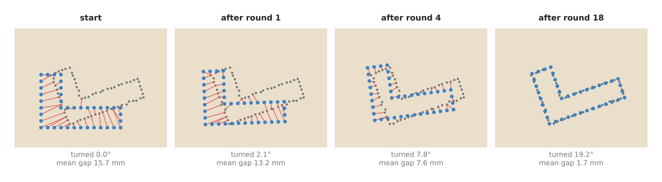
So after one round the model has barely turned, after four rounds it is part of the way there, and after 18 rounds it sits on the scan.
The table below gives the numbers after some of the rounds, and each row is one round. In it, "Turned" and "shifted" are the model's total movement since the start, while the real answers are 20° and (30, 20) mm.
| Round | Mean gap (mm) | Turned | Shifted (mm) |
|---|---|---|---|
| 0 (start) | 15.74 | 0.00° | (0.0, 0.0) |
| 1 | 13.16 | 2.14° | (5.3, 6.5) |
| 2 | 11.05 | 4.15° | (8.6, 11.3) |
| 4 | 7.62 | 7.77° | (15.8, 17.4) |
| 8 | 3.80 | 14.14° | (24.7, 20.6) |
| 12 | 1.91 | 18.33° | (28.5, 20.0) |
| 17 | 1.70 | 19.18° | (30.0, 20.3) |
| 18 | 1.70 | 19.18° | (30.0, 20.3) |
ICP also needs a rule for when to stop. The rule here is to stop when the mean gap falls by less than 0.001 mm in one round, which happened after round 18. Real libraries use the same kind of rule, and they add a largest number of rounds, such as 30 or 50, so that ICP always ends whatever the scan looks like.
The picture below plots the mean gap after each round of this run.
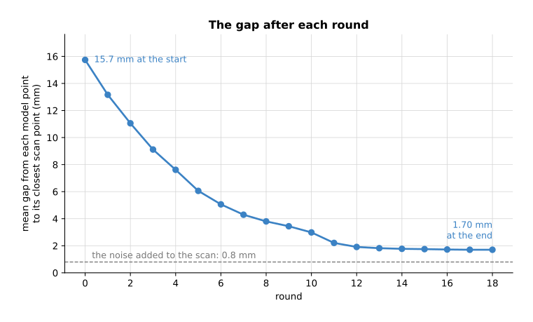
The gap falls fast for the first twelve rounds, then hardly changes, and that is when the stop rule ends the loop.
The answer ICP reaches is 19.2° instead of 20°, and (30.0, 20.3) mm instead of (30, 20) mm. As a result, it is close but not exact, and there are two reasons for that. The first reason is that the scan's points carry noise. The second reason is that the model's points and the scan's points do not sit at the same places along each edge, because one set is spaced 10 mm apart and the other 6 mm. So even at the right pose, each model point's closest scan point is up to 3 mm along the edge from it. This is also why the mean gap ends at 1.70 mm rather than at the 0.8 mm of noise.
2.5 The pseudocode#
The two steps above, together with the stop rule, are written out below in plain steps rather than in any real programming language.
icp(model_points, scan_points, first_guess, max_rounds, stop_change, max_pair_distance):
    pose = first_guess
    moved = model_points moved by pose
    previous_gap = infinity
    repeat up to max_rounds times:
        # step one: pairs
        pairs = empty list
        for each point m in moved:
            s = nearest point to m in scan_points          # use a k-d tree built once
            if distance(m, s) <= max_pair_distance:
                add (m, s) to pairs
        gap = mean distance over pairs
        if previous_gap - gap < stop_change: stop
        previous_gap = gap

        # step two: best move for these pairs
        cm = centroid of the m's in pairs
        cs = centroid of the s's in pairs
        R  = the rotation that best lines up (m - cm) with (s - cs)   # SVD
        t  = cs - R * cm
        moved = R * moved + t
        pose  = (R, t) combined with pose
    return pose, gap
The scan does not move during the loop, so its k-d tree is built once, before
the first round. The max_pair_distance test then throws away pairs that are
too far apart to be real. That test matters when the scan also holds other
things, such as the table or a neighbouring part.
2.6 Point-to-plane: a faster version#
The version above is called point-to-point ICP, because it measures the gap from each model point to one scan point. But that measure is slow when a surface can slide along itself, which is why the long flat edges of the bracket took many rounds to slide into place in the example.
Point-to-plane ICP measures the gap from each model point to the flat surface through its partner instead. That surface is set by the partner's normal , which is the direction straight out of the surface. With this measure a model point that slides along the right surface costs nothing. So ICP spends its moves only on the direction that matters, and it usually needs far fewer rounds. However, it needs normals for the scan, which means one more k-nearest search per scan point before ICP starts, and both Open3D and PCL provide the method.
3. Where it is used on a robot arm#
Because ICP sharpens a pose rather than finding one from nothing, it is used on a robot arm wherever the arm already has a rough idea of where something is and needs an exact one. The list below gives the common jobs, and each one supplies that rough idea in a different way.
- Finding the exact pose of a known part. A detector or a simple rule finds roughly where a part lies in a bin. ICP then lines the part's computer-aided design (CAD) model up with the depth scan, and gives a pose accurate enough to grip it at a chosen spot. The robot-arm project v5-pick-glasses lists matching against known glass models with Open3D's ICP as one of its approaches.
- Finishing a learned pose. A learned pose model, such as those in Book 7's keypoints and object pose, gives a pose that is often a few millimetres or a few degrees off. A few rounds of ICP from that pose fix the last part of the error. This is a common pairing: the learned model gives the first guess, and ICP gives the precision.
- Joining several views into one cloud. A camera on the wrist takes pictures from several arm poses, and the arm's joint readings say roughly where the camera was for each picture. ICP then lines each new cloud up with the ones before it, to remove the small errors left by calibration and by the joints.
- Following a part that moves a little. When a part is being pushed or is in the gripper, its pose in one frame is a good first guess for the next frame. ICP from that guess follows the part with a small number of rounds per frame.
- Checking a placement. After the arm sets a part down, a scan and ICP against the model say where the part actually ended up. If the pose differs from the planned one by more than a limit, the robot can try again.
- Checking calibration. If the camera-to-arm calibration is right, a scan of a known object at a known place lines up with its model with almost no movement. If ICP has to move it by several millimetres, the calibration has drifted. The calibration page explains the calibration itself.
4. Where it is useful, and where it is not#
All the jobs in section 3 rely on ICP being precise, which it is whenever it starts close to the answer. The danger is that ICP always returns an answer, even when that answer is wrong. It stops as soon as the gap stops shrinking, and the gap can stop shrinking at a wrong pose.
The picture below shows what that looks like, with the same bracket scanned twice, once turned 20° and once turned 120°. So ICP starts from the same first guess in both runs.
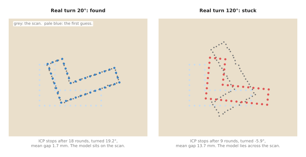
From 20° away ICP finds the bracket, and it also found it from 45°, 60° and 90° away, after 25 to 36 rounds. From 120° away, however, it stops after 9 rounds with the model turned −5.9° and lying across the scan. Its mean gap there is 13.7 mm, against 1.7 mm for the good result. That difference is the sign to watch for, because a final gap much bigger than the camera's noise is what a wrong pose looks like. Such a stuck answer is called a local minimum, which is a pose from which every small move makes the gap worse, although it is not the best pose overall.
The table below lists the common problems. Read each row as: what goes wrong, the sign you see, and what people use instead.
| Problem | The sign you see | What people use instead |
|---|---|---|
| The first guess is too far off. How far is too far depends on the shape: the diagram script's bracket was found from 90° away, but not from 100° | the final gap is much larger than the camera noise | a global method first, such as random sample consensus (RANSAC) on matched surface features, as section 5 shows, or several ICP runs from different starting turns, keeping the best |
| The part is symmetric, such as a cylinder or a square plate | the gap is small, but the turn about the symmetry axis is random from run to run | accept that the turn is unknown, or use colour or a marking, as in coloured ICP |
| The scan also holds the table or other parts | the model is pulled towards the table or a neighbour | cut the part out of the scan first, and reject pairs further apart than a limit |
| Only part of the object is visible | the model slides to cover the missing side | reject far pairs; use a model of only the side the camera can see |
| A large flat surface, such as a box lying on a table | the model slides along the surface and never settles, or settles in the wrong place along it | point-to-plane ICP helps with speed; a feature such as an edge or a hole is needed to fix the position |
| The model is in millimetres and the scan in metres | a nonsense answer after one round | check the units before calling ICP |
| Many rounds on large clouds | ICP is too slow for the camera rate | downsample both clouds to a point every few millimetres first; use point-to-plane |
5. Getting a first guess: 3D features and global registration#
Section 4 showed that ICP needs a first guess close to the answer. So this section shows how a program can get one from the scan alone, with no idea at all where the part is or which way it is turned. The method is called global registration, in which "registration" means lining two point sets up. The word "global" means that the method searches every possible pose rather than only the poses near a guess.
Global registration does for depth scans what image features and matching does for pictures, and it does so in the four steps below.
- Work out which way the surface faces at every point. This direction is the point's normal.
- Describe the shape round every point as a short list of numbers, called a local 3D feature.
- Pair each model point with the scan point whose feature is most alike, and keep the pairs that agree on one rigid move, with RANSAC.
- Use that rough move as ICP's first guess.
The example here is the case where ICP failed in section 4, which is the bracket
turned 120°. The numbers come from docs/diagrams/searching_and_matching_2.py,
which runs every one of these steps. As before, the example is flat so that it
fits on a page, and section 5.5 says what changes in 3D.
5.1 Surface normals#
The first of those four steps is to find a normal, which is the direction straight out of a surface, at right angles to it. A single point on its own has no direction, so the program looks at the point's neighbours instead. It finds the point's 5 nearest neighbours with a nearest-neighbour search , and it fits the straight line that passes closest to them and to the point itself. Then it takes the direction at right angles to that line. In 3D it fits a flat plane instead of a line, so the normal is the direction at right angles to that plane. The fit uses principal component analysis (PCA), a standard method that finds the direction in which a set of points is spread out most and the direction in which it is spread out least. That is why the normal is the direction of least spread.
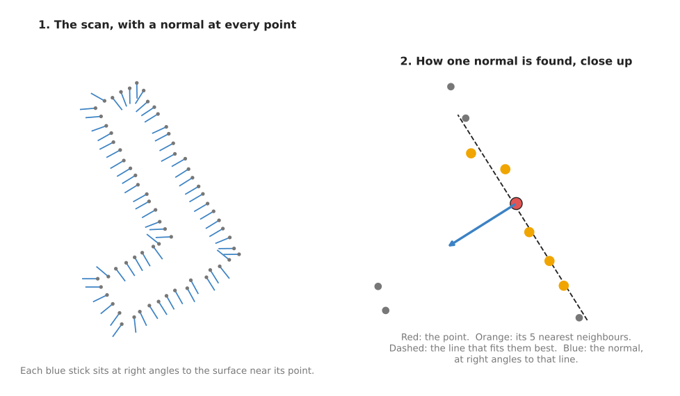
The left panel shows the normal at every point of the scan, and on the straight edges those normals are neat and parallel. At the corners they point at an angle, because the neighbours there come from both edges. The fit cannot tell "out of the part" from "into the part", so a normal can point either way. Real programs therefore turn every normal to face the camera, because a camera can only see surfaces that face it. The feature described below ignores which way a normal points, so it does not need that step.
5.2 Local 3D features#
Every point now has a normal, but a normal only says which way a surface faces, and many points on the same part face the same way, so a normal on its own cannot tell those points apart. To tell them apart, the program describes the shape of the whole neighbourhood round each point. The best-known description of that kind is the fast point feature histogram (FPFH). For one point, FPFH looks at every neighbour within a set radius. For each of those neighbours it measures, in three angles, how the neighbour's normal is turned relative to the point's own normal. It then counts how many neighbours fall into each range of angles. Those counts form a histogram, which is a row of bins, with each bin holding how many things fell into it. FPFH has 33 bins in all, and because each bin describes part of the shape round the point, two points on similar shapes, such as two sharp edges, get similar histograms. However, a point on a flat surface gets a very different histogram.
The diagram script uses a smaller feature of the same kind, with 9 bins, so that it can be drawn on the page. For each point it looks at every neighbour within 45 mm. It then sorts each neighbour by distance (near, up to 15 mm; middle, 15 to 30 mm; far, 30 to 45 mm), and also by the angle between the two normals (same way, up to 30°; tilted, 30° to 60°; across, 60° to 90°). Each bin then holds the share of neighbours that fell into it.
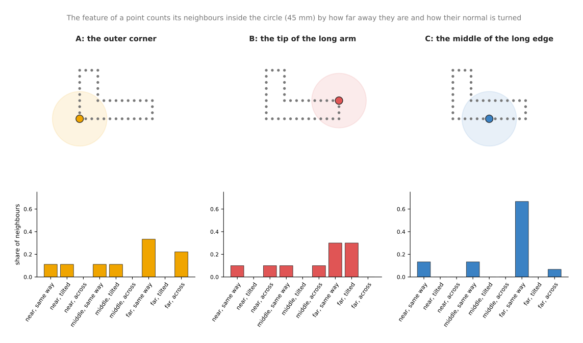
Point C, in the middle of the long edge, has two thirds of its neighbours in "far, same way", because the edge there is straight. Point A, at the outer corner, has neighbours on two edges at right angles, so a share of them falls in "far, across". Point B, at the tip of the long arm, sees the short end of the arm and the inner edge, and so it has a different mix again. Points along the middle of a straight edge therefore all look alike, which is why the corners and the arm ends are what make the bracket recognisable.
A second well-known kind of feature is the point pair feature (PPF), which describes two points at a time rather than one. For two points with normals it stores four numbers: the distance between them, the angle between each normal and the line joining them, and the angle between the two normals. Here is one such feature, computed in 3D for two points on a box. Point one is on the top face, at (0, 0, 50) mm, with its normal pointing up, while point two is on a side face, at (40, 0, 20) mm, with its normal pointing sideways. For that pair the four numbers are 50.0 mm, 126.9°, 36.9° and 90.0°, and they stay the same wherever the box is and however it is turned. A program therefore stores the four numbers for every pair of points on the model in a table. In the scan, each pair of points then looks itself up in that table, and every model pair it matches votes for a pose, so the pose with the most votes wins.
5.3 Matching features, then RANSAC#
Once every point has a feature, the program pairs each model point with the scan point whose feature is most alike. This is again a nearest-neighbour search, but among features instead of among positions. Most of these pairs are wrong, because edge points all look alike, and in the example only 5 of the 40 pairs lie within 5 mm of the right scan point.
RANSAC does not mind that most of the pairs are wrong, because it repeats the steps below many times and keeps only the move that the most pairs agree with.
- Pick two pairs at random. In 3D it picks three.
- Check that the two model points are about as far apart as the two scan points. If not, at least one pair is wrong, so the try is skipped at once. This cheap check saves most of the work.
- Compute the rigid move that fits the two pairs, with the method of section 2.3.
- Count the pairs that the move brings within 5 mm of each other.
- Remember the move with the most such pairs.
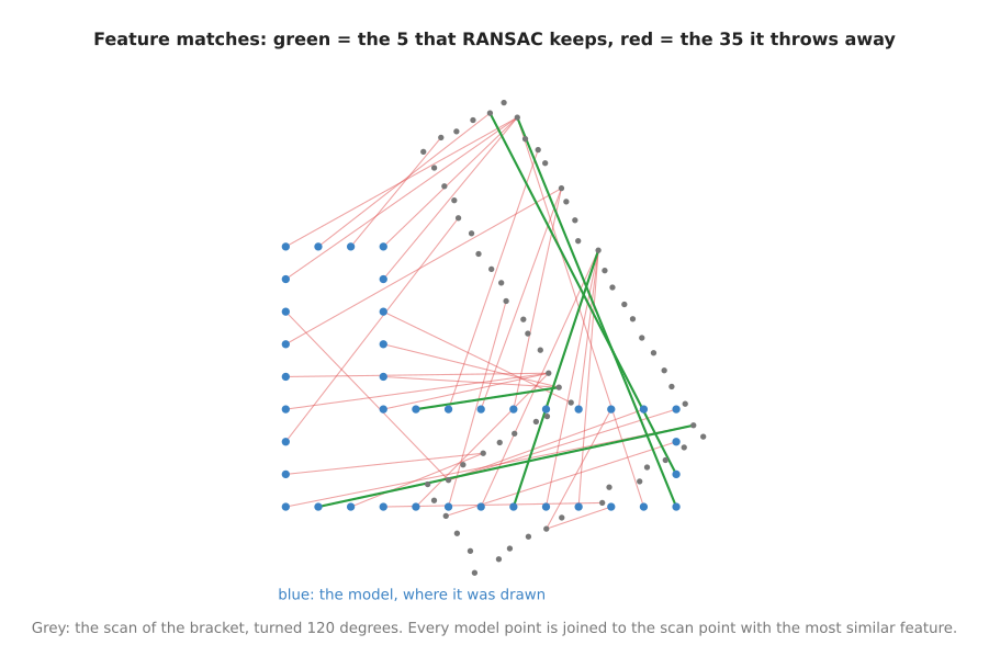
In the example, RANSAC found a move that 5 pairs agree with on its 90th try out of 500, and those 5 pairs are the green lines in the picture. Every one of the 35 red pairs is thrown away, because it does not agree with that move. Five right pairs out of forty is a small share. So two pairs picked at random are both right only about once in 64 tries, which is why it took 90 tries.
Fast global registration (FGR) is a common alternative to RANSAC for this step, and it does not pick random pairs at all. Instead, it fits one move to all the pairs at once, then repeats the fit while giving the pairs that disagree with the move less and less weight. In practice it is usually faster than RANSAC, and it gives the same kind of rough answer.
5.4 Finishing with ICP#
The move from RANSAC rests on a handful of pairs, so it is only rough, and ICP is what then makes it exact. The picture below compares three results for the bracket turned 120°.
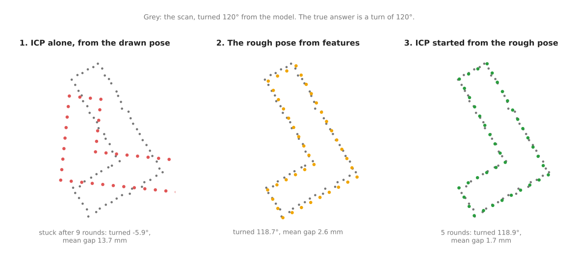
The table below gives the numbers for those three results, and each row is one way of finding the pose. The right answer, for comparison, is a turn of 120° and a shift of (30, 20) mm.
| Method | Rounds of ICP | Turned | Mean gap (mm) |
|---|---|---|---|
| ICP alone, from the drawn pose | 9 | −5.9° | 13.7 |
| Features and RANSAC, no ICP | 0 | 118.7° | 2.6 |
| Features and RANSAC, then ICP | 5 | 118.9° | 1.7 |
The feature pose alone is already within about 1.3° of the right turn. So ICP starting from there needs only 5 rounds, where it needed 18 rounds from a 20° start in section 2.4. The final answer is 1.1° from 120°, and the part's centre moved by (30.2, 19.2) mm. But it stops short of the exact answer for the same reason as in section 2.4, which is that the model points and the scan points sit at different places along each edge. The final mean gap, 1.7 mm, is the same as in the good result of section 4, and that sameness is the sign that the answer is right.
5.5 Where it is used, where it fails, and libraries#
Everything above works the same way in 3D, with three changes. The first is that the normal comes from a plane fitted to the neighbours rather than from a line. The second is that RANSAC picks three pairs at a time rather than two. The third is that the clouds are first downsampled, which means thinning them to one point every few millimetres, because computing a feature for every one of 300,000 camera points is slow.
On a robot arm, global registration is used in the places listed below.
- Picking a known part that can lie any way up. A part in a bin may be on its side or upside down. No first guess is good enough for ICP alone. Global registration gives the rough pose, and ICP gives the precise one.
- Getting going again after tracking is lost. When the arm follows a part with ICP from frame to frame and the part is knocked, the old pose is no longer a good guess. Global registration finds the part again from nothing.
- Joining two scans with no idea how the camera moved. For example, two scans from two fixed cameras before they are calibrated to each other.
- Checking an ICP result. If ICP from the previous pose and global registration disagree, one of them is wrong, and the arm should not grip yet.
It also fails in ways that are easy to predict, and the table below lists them, where each row gives what goes wrong, the sign you see, and what people use instead.
| Problem | The sign you see | What people use instead |
|---|---|---|
| The part has few distinct shapes, such as a flat box or a ball | few RANSAC inliers, and a pose that changes from run to run | colour or texture, from image features, or a learned pose model |
| The normal and feature radius do not suit the scan: too small for the camera's noise, or too large for the part | features are noise, and almost no pairs are right | set the normal radius to a few times the point spacing, and the feature radius to a few times that |
| The part is a small share of a cluttered scan | RANSAC fits the move to the table or a neighbouring part | cut the part out of the scan first, for example with clustering |
| The part is symmetric | the pose flips between look-alike turns | accept the ambiguity, or use a marking that breaks the symmetry |
The table below lists the functions to look up, with one row for each library.
| Library | Languages | Functions or classes |
|---|---|---|
| Open3D | Python, C++ | PointCloud.estimate_normals; open3d.pipelines.registration.compute_fpfh_feature; registration_ransac_based_on_feature_matching, with CorrespondenceCheckerBasedOnEdgeLength for the distance check in step 2 above; registration_fgr_based_on_feature_matching |
| Point Cloud Library (PCL) | C++ | pcl::NormalEstimation, pcl::FPFHEstimation, pcl::SampleConsensusPrerejective |
| OpenCV (contrib) | C++, Python | cv::ppf_match_3d::PPF3DDetector, the point pair feature method, in the surface_matching module |
| TEASER++ | C++, Python | a global registration method that stays right even when almost all feature pairs are wrong |
6. Libraries that provide it#
You do not have to write any of this yourself, because ICP is part of every major point cloud library. The table below lists the well-known ones, and its "function or class" column gives the name to look up in each library's documentation.
| Library | Languages | Function or class | Note |
|---|---|---|---|
| Open3D | Python, C++ | open3d.pipelines.registration.registration_icp, with TransformationEstimationPointToPoint or TransformationEstimationPointToPlane | also has coloured ICP, and global registration with RANSAC on features |
| Point Cloud Library (PCL) | C++ | pcl::IterativeClosestPoint, pcl::GeneralizedIterativeClosestPoint | the generalised version models each point as a small patch of surface |
| OpenCV (contrib) | C++, Python | cv::ppf_match_3d::ICP, in the surface_matching module | paired in that module with a global matcher for a first guess |
| trimesh | Python | trimesh.registration.icp | small and easy; aligns points to a mesh |
| Eigen | C++ | Eigen::umeyama | only the best-move step (section 2.3), for writing your own ICP |
Book 3's tools and libraries explains where Open3D fits into a robot arm's software.
7. Why ICP, and what it costs#
The method, its failures and its libraries are now all covered. As a result, this section answers the four standing questions: what the technique is, what it does for you, why it rather than the obvious alternative, and what it costs.
ICP moves a model point set onto a scanned point set by pairing closest points and fitting a rigid move, over and over. So it turns a rough pose into an exact one, often to within a millimetre or a degree, using only the shape of the part.
The obvious alternative is to try every pose: every turn in steps of one degree and every shift in steps of one millimetre, and keep the pose with the smallest gap. In 3D that is millions of poses, each checked against the whole scan, which is far too slow for a robot. The second alternative is to match distinctive features, such as corners, between the model and the scan, and fit the pose to those matches with RANSAC. Feature matching does not need a first guess, which is its great advantage, but it is less exact, because it uses only a few points. That is why the usual answer is to use both: features for the first guess, then ICP to make it exact, as section 5 shows.
ICP costs you several things, starting with a first guess. Because it gives a confident wrong answer when that guess is poor, you must check the final gap. It also needs a model of the part, which means a CAD file or an earlier scan. And it needs a clean scan, with the table and other objects cut away. Because it runs a nearest-neighbour search for every model point in every round, it needs downsampled clouds to run at camera rate. Finally, it cannot tell apart the poses that a symmetric part makes look the same.
8. The learned alternative#
The last alternative to weigh is a learned one, and Book 7's keypoints and object pose describes networks that give an object's pose directly from a picture. Models such as MegaPose and FoundationPose need only the part's CAD model, or for FoundationPose a few photos of it. Because they cope with clutter and need no first guess, they can take the place of the 3D features and RANSAC in section 5. Once the part has been found, FoundationPose can also follow its pose from frame to frame, which is the job ICP does from the last pose. Then there are networks that read point clouds, from Book 7's point cloud models , which can learn their own 3D features in place of hand-written ones. But a pose model needs a graphics processor, and it gives no warning when it is wrong. So ICP is still run after it, as section 3 describes, and ICP's final gap is the check. That is why ICP alone still wins when a first guess is already at hand, such as the last frame's pose or a part in a fixed tray.
9. Where to read next#
- Nearest-neighbour search is the search inside every ICP round.
- Rigid transforms explains the rotation and shift that ICP returns, and how to chain it with the camera's pose to get the part's pose in the arm's frame.
- RANSAC gives a first guess that does not need to be close.
- Least-squares fitting explains "the smallest sum of squared distances", the measure ICP's best-move step uses.
- Book 7's scene reconstruction builds a 3D scene from many views with learning.
- Image features and matching finds a first guess from a camera picture instead of a depth scan, for parts with printing or texture.
- Assignment and matching pairs whole objects rather than points, with a strict one-to-one rule that ICP does not have.
10. Using it in Python#
Section 2 ran the pair-and-move loop by hand, section 5 covered how to get the first guess, and section 6 named Open3D as the usual library in Python. This section shows the Open3D call, because ICP is a case where the whole algorithm is one function and the difficulty has moved entirely into its arguments. After reading it you should be able to align a model with a scan and, just as importantly, to tell whether the answer it gave is worth using.
The code below loads a stored model of a part and a scan of the real part, thins both, and then runs ICP.
import numpy as np
import open3d as o3d

model = o3d.io.read_point_cloud("bracket_model.ply")
scan = o3d.io.read_point_cloud("bracket_scan.ply")

# Thinning both to one point per 3 mm cube makes each round faster and the
# distances more even, which is what ICP assumes.
model = model.voxel_down_sample(voxel_size=0.003)
scan = scan.voxel_down_sample(voxel_size=0.003)
scan.estimate_normals(o3d.geometry.KDTreeSearchParamHybrid(radius=0.01, max_nn=30))

first_guess = np.eye(4)
first_guess[:3, 3] = [0.30, -0.05, 0.02]   # from a detector, or from a fixture

result = o3d.pipelines.registration.registration_icp(
    model, scan,
    max_correspondence_distance=0.01,      # metres: ignore pairs further apart
    init=first_guess,
    estimation_method=o3d.pipelines.registration.TransformationEstimationPointToPlane(),
    criteria=o3d.pipelines.registration.ICPConvergenceCriteria(max_iteration=50))

print(result.fitness, result.inlier_rmse)   # how much overlapped, how well it fitted
T_scan_model = result.transformation
The library does all of section 2 for you. Every round it runs the
nearest-neighbour search of the previous page, throws away the pairs that are
further apart than max_correspondence_distance, computes the best rigid move for
the pairs that are left, applies it, and stops when the improvement falls below
relative_fitness or relative_rmse, or when it has done max_iteration rounds.
Choosing TransformationEstimationPointToPlane switches to the point-to-plane
variant, which usually converges in fewer rounds on surfaces and is why the code
estimates normals on the scan first.
What you still write yourself is the first guess and the verdict. ICP has no way to
find a pose, only to improve one, so the first_guess comes from somewhere else:
the middle of a cluster, a detected marker, the known position of a fixture, or the
global registration of section 5, which in Open3D is
compute_fpfh_feature followed by
registration_ransac_based_on_feature_matching. You also write the check, because
registration_icp always returns a transform and never raises an error when the
answer is nonsense. The two numbers to check are fitness, which is the fraction
of model points that found a partner and which should be near 1 for a part you can
see fully, and inlier_rmse, which should come out near your camera's noise rather
than several times larger.
What you have to decide or measure is three numbers, and all three are physical.
voxel_size is how coarse to thin the clouds, and 2 to 5 mm is usual for a
table-top part, because thinning speeds up every round and stops the dense parts of
the scan from dominating. max_correspondence_distance is the pair-rejection
distance and it is the argument that matters most: set it to a few times the depth
camera's noise, and start it larger when the first guess is poor and shrink it once
the model is close. max_iteration is a time budget rather than an accuracy
setting, since a run that has not converged in 50 rounds is usually one whose first
guess was wrong, and section 4 lists the other signs of that.