This page explains nearest-neighbour search: given a set of points and one more point, find the point in the set that is closest to it. It answers four questions, the first of which is this: how do you find the nearest point without measuring the distance to every point? What is a k-d tree, and how is it built and searched? What are the k-nearest and radius versions of the search for? And where does a robot arm use all of this?
It is for a reader who knows what a point and a point cloud are, from Books 1 and
2, and who has read the chapter overview. So no algorithms
course is needed to follow it. Instead, every step is shown with a small example
on a table top, with real numbers from the diagram script
docs/diagrams/searching_and_matching.py, which builds and searches a real k-d
tree.
Nearest-neighbour search is the most used technique in this chapter, because the other two pages, iterative closest point and assignment and matching, both call it.
Contents#
- The idea in one sentence
- How it works, step by step · Brute force: measure every distance · Building a k-d tree · Searching the tree · The k nearest, and everything within a radius · The pseudocode
- Where it is used on a robot arm
- Where it is useful, and where it is not
- Libraries that provide it
- Why a k-d tree, and what it costs
- The learned alternative
- Where to read next
- Using it in Python
1. The idea in one sentence#
Nearest-neighbour search finds the point in a set that is closest to a given point, and a k-d tree makes that fast by cutting space into boxes, so that most boxes can be skipped without looking inside them.
The given point is called the query, and "closest" usually means the ordinary straight-line distance, which is called the Euclidean distance. So, for two points on a table at (x1, y1) and (x2, y2), that distance is the square root of (x1 − x2)² + (y1 − y2)².
Here is an everyday example, in which you are in a strange town and want the nearest chemist. You could look up the address of every chemist in the country and work out how far each one is, but nobody does that. Instead, you look only at the part of the map around you, because a chemist in another town cannot be the nearest one. This is what a k-d tree lets a computer do: it looks only at the parts of space that could hold the answer.
2. How it works, step by step#
That is why the rest of this section works that idea through on a table that is 600 mm wide and 400 mm deep, seen from above. Eleven objects stand on it, named A to K, and the gripper tip is above the table at (430, 300) mm. So the question is which of those eleven objects is nearest to the gripper.
The positions of the eleven objects are listed below in millimetres, with one column per object.
| Object | A | B | C | D | E | F | G | H | I | J | K |
|---|---|---|---|---|---|---|---|---|---|---|---|
| x | 60 | 120 | 180 | 250 | 300 | 360 | 400 | 460 | 500 | 540 | 220 |
| y | 300 | 80 | 220 | 350 | 150 | 60 | 270 | 340 | 130 | 240 | 40 |
The example is flat, with two numbers per point, so that it fits on a page. While a point cloud from a depth camera has three numbers per point, x, y and z, every step below works the same way in three dimensions. As a result, nothing is lost by drawing the example flat.
2.1 Brute force: measure every distance#
The simplest way to answer that question measures the distance from the query to every point and keeps the smallest. This is called brute force, because it uses no cleverness, only work.
The picture below shows the 11 distances, one from the gripper to each of the objects.
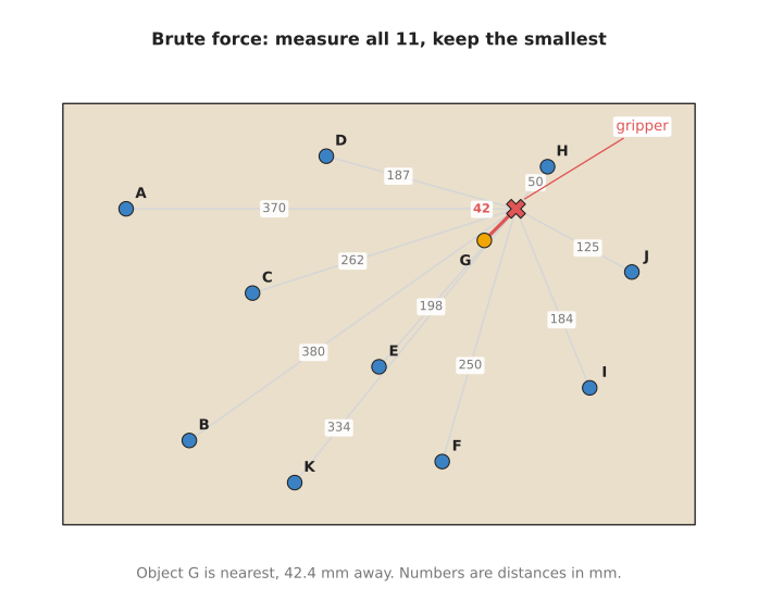
Object G, at (400, 270), is nearest, and its distance is the square root of 30² + 30², which is 42.4 mm. Then comes H, the second nearest, at 50.0 mm.
Brute force is always right, and for 11 points it is also fast, because it needs one distance check per point. So for one query against n points, that is n checks. The trouble starts when there are many points and many queries. For example, matching every point of one 3,000-point scan to its nearest point in another needs 3,000 × 3,000 = 9,000,000 checks.
2.2 Building a k-d tree#
Those 9,000,000 checks are what a k-d tree avoids, because it is a way of storing points so that a search can skip most of them. The name is short for "k-dimensional tree", in which k is the number of coordinates each point has. So that is 2 on this flat table, and 3 for a point cloud.
The tree is built by cutting the space in two, again and again.
- Sort the points by x and take the middle one, then draw a line through it, across the x direction, so that every point with a smaller x goes to the left side and every point with a larger x goes to the right side.
- On each side, sort the points by y, take the middle one, and cut across the y direction through it.
- Keep going, switching between x and y at each level (x, y, z in 3D), until every point has its own cut.
For the table, step 1 sorts the 11 points by x, and the middle one of 11 is the sixth, which is E at x = 300. That is why the first cut is the line x = 300. Then A, B, C, D and K go to the left side, and F, G, H, I and J go to the right side.
Step 2 then works on each side, and on the left, sorted by y, the points are K (40), B (80), C (220), A (300), D (350). The middle one is C, so the left side is cut at y = 220. On the right, sorted by y, the points are F (60), I (130), J (240), G (270), H (340). Once again the middle one is J, so the right side is cut at y = 240.
After that, the third level cuts by x again, and so on, until every point has its own cut. The picture below shows the result: the table cut into boxes on the left, and the same cuts drawn as a tree on the right.
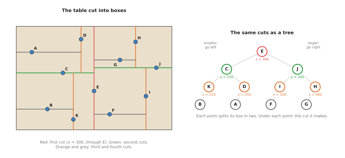
Each circle in the tree is one point, and it owns one cut. So its left branch holds the points on the smaller side of that cut, and its right branch holds the points on the larger side. E is at the top, because it made the first cut, and the tree is four levels deep.
Building the tree takes some work, because each level sorts the points. But it is done once, and after that every search uses the same tree.
2.3 Searching the tree#
Once the tree is built, the search walks down it towards the query and then walks back up again. On the way back, it only looks at a box if that box could hold something nearer than the best point found so far.
For the gripper at (430, 300), the search goes like this.
- Check E: the distance is 198.5 mm, which is the best so far, and the gripper's x of 430 is more than E's 300, so go to the right branch.
- Check J: 125.3 mm, which is the new best, and the gripper's y of 300 is more than J's 240, so go to J's upper branch.
- Check H: 50.0 mm, which is the new best again, and the gripper's x of 430 is less than H's 460, so go to H's left branch.
- Check G: 42.4 mm, which is the new best, and G has no branches, so the walk down is over.
Now the search walks back up and asks, at each cut, whether the other side is worth a look.
- At H, the other side is empty, so nothing there needs checking.
- At J, the other side is everything below y = 240, and the gripper is at y = 300, so anything below that line is at least 300 − 240 = 60 mm away. Since the best so far is 42.4 mm, nothing on that side can beat it, and I and F are skipped without measuring them.
- At E, the other side is everything left of x = 300, and the gripper is at x = 430, so anything there is at least 130 mm away. That means all five points there, A, B, C, D and K, are skipped.
The answer is G at 42.4 mm, the same as brute force, but the search measured 4 distances instead of 11. The picture below shows the order of the checks, and the boxes that were skipped.
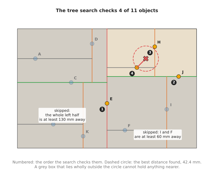
The dashed circle has the radius of the best distance found. Since a grey box lies wholly outside that circle, it cannot hold anything nearer than the point already found.
The saving grows with the number of points, and the diagram script measured that saving on a real pair of scans. Matching every point of a 3,000-point scan to a second scan took 44,425 checks with the tree, about 15 per query, against 9,000,000 by brute force. As a rule of thumb, a search in a well-balanced tree of n points checks a number of points that grows like the number of times you can halve n, not like n itself.
2.4 The k nearest, and everything within a radius#
The search described so far returns a single point, and two variants of it are used as often as that plain one.
k-nearest-neighbour search returns the k closest points instead of one. The walk through the tree is the same, except that it keeps a list of the k best points found so far. Then it skips a box only if the box is further away than the worst of those k.
Radius search returns every point within a set distance of the query, for example every point within 40 mm. As a result, this time the search skips a box only if the box is further away than the radius.
The two answer different questions, and the picture below shows the difference on a cloud that is crowded on the left and thin on the right.
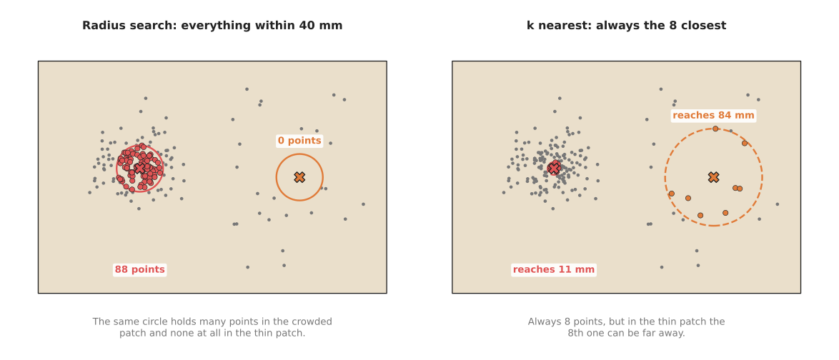
In the crowded patch, a 40 mm radius holds 88 points, and the 8 nearest points all lie within 10.9 mm. In the thin patch, the same radius holds no points at all, and the 8 nearest points reach out to 83.6 mm.
So use k nearest when you need a fixed number of points, for example at least a few points to fit a plane through. Use a radius instead when the distance itself means something, for example "points closer than 5 mm belong to the same object". Some libraries also offer a mix of the two: the k nearest, but none further than a radius.
2.5 The pseudocode#
The steps above are easier to follow as code, so the pseudocode below is written in plain steps, not in any real programming language. "axis" means x at the top level, y at the next, and so on, switching at each level.
build_tree(points, depth):
    if points is empty: return nothing
    axis = depth mod (number of coordinates)
    sort points by their value on axis
    middle = the point in the middle of the sorted list
    node.point = middle
    node.axis  = axis
    node.left  = build_tree(points before middle, depth + 1)
    node.right = build_tree(points after middle,  depth + 1)
    return node

nearest(node, query, best):
    if node is nothing: return best
    d = distance(node.point, query)
    if best is nothing or d < best.distance:
        best = (node.point, d)
    gap = query[node.axis] - node.point[node.axis]
    if gap < 0: near_side = node.left,  far_side = node.right
    else:       near_side = node.right, far_side = node.left
    best = nearest(near_side, query, best)
    if absolute value of gap < best.distance:
        best = nearest(far_side, query, best)     # the far side might hold something nearer
    return best

radius_search(node, query, r, found):
    if node is nothing: return
    if distance(node.point, query) <= r: add node.point to found
    gap = query[node.axis] - node.point[node.axis]
    if gap > -r: radius_search(node.right, query, r, found)   # the larger side is within reach
    if gap <  r: radius_search(node.left,  query, r, found)   # the smaller side is within reach
The first call is nearest(root, query, nothing), and the one line that makes
the tree fast is the test absolute value of gap < best.distance. When that
test is false, the whole far side is skipped without a single distance being
measured.
3. Where it is used on a robot arm#
As the sections above suggest, nearest-neighbour search sits inside many other steps, and these are the common places on a robot arm.
- The surface direction at each point of a cloud. To grip a mug, the arm needs to know which way its surface faces at the grip point, and that direction is called the normal. The software takes the 20 or 30 nearest points around a point, fits a small flat patch through them, and takes the direction straight out of the patch. This is done for every point of the cloud, so it needs one k-nearest search per point.
- Growing clusters of points into objects. After the table plane is removed, the points that are left belong to the objects on it. A radius search then groups every point with the points within, say, 10 mm of it, and those groups with their neighbours, until each group is one object. The clustering page covers this, and Book 2 shows it in removing the plane, then clustering.
- Removing stray points. A depth camera gives some points that float in the air, away from any surface, so a point whose nearest neighbours are all far away is probably one of these and can be removed.
- Aligning a model to a scan. Every round of iterative closest point finds, for each model point, the nearest scan point.
- Matching a detection to a known object. When a camera sees an object and the software keeps a list of objects it already knows, the nearest known object is the first guess of which one it is. The assignment and matching page shows when that first guess goes wrong.
- Choosing the nearest object to pick, or the nearest free spot to place. A robot clearing a table often takes the object nearest to the gripper first, to keep each move short. The robot-arm project v5-pick-glasses sorts the glasses by their distance from the robot base and picks the nearest one first.
- Looking up a stored answer. Some programs store many past situations with the action that worked, for example a grasp for each of 500 known object shapes. For a new object, they describe it with a list of numbers and look up the nearest stored one, so here the "points" have many coordinates, not three.
- Checking a planned path for collisions. A motion planner asks, for many points along the arm, "how far is the nearest obstacle point?", and a k-d tree over the obstacle cloud answers each of these quickly. The sampling-based planning page also uses nearest-neighbour search to find the nearest node already in its tree.
4. Where it is useful, and where it is not#
In all of those places, nearest-neighbour search is exact and fast, as long as the points have only a few coordinates. For example, a position on this table has two coordinates, and a point in a cloud has three. The search has limits, though, and each limit shows up in a way you can recognise.
The table below lists the common problems, one per row. Read each row as: this is what goes wrong, this is the sign you see, and this is what people use instead.
| Problem | The sign you see | What people use instead |
|---|---|---|
| The nearest point is still far away | a matched point is 50 mm away when the objects are 20 mm apart | a maximum distance: reject any match further than a set limit |
| Many coordinates per point, such as 33 or 128 numbers describing a patch of surface | the tree search is barely faster than brute force | an approximate search, as in FLANN or FAISS, which is allowed to miss the true nearest point now and then |
| The cloud changes every frame | building a new tree each time takes longer than the searches | a voxel grid (the space cut into equal cubes), or brute force on a graphics card |
| Points have very different densities | a fixed radius returns hundreds of points in one place and none in another | k nearest, or the mix of k nearest and a radius |
| x, y and z measure different things, such as position in metres and colour from 0 to 255 | the "nearest" point is decided almost only by the colour | scale each coordinate so that they are comparable before building the tree |
| Only a few points and a few queries | the tree takes longer to build than brute force takes to answer | brute force; it is simpler and fast enough below a few hundred points |
The second row needs a word of explanation, because in two or three dimensions a box that is far from the query is easy to skip. With 128 coordinates, almost every box is close to the query along at least one coordinate, so almost none can be skipped. The tree then checks nearly every point, and its extra work makes it slower than brute force.
5. Libraries that provide it#
None of this has to be written from scratch, because almost every point cloud and maths library has a k-d tree. So you very rarely need to write one yourself. The table below lists well-known ones, and the "function or class" column gives the name to look up in each library's documentation.
| Library | Languages | Function or class | Note |
|---|---|---|---|
| SciPy | Python | scipy.spatial.KDTree (query, query_ball_point) | the easiest start in Python; exact search |
| scikit-learn | Python | sklearn.neighbors.NearestNeighbors, KDTree, BallTree | chooses brute force or a tree for you |
| Open3D | Python, C++ | open3d.geometry.KDTreeFlann (search_knn_vector_3d, search_radius_vector_3d, search_hybrid_vector_3d) | the hybrid search is the "k nearest within a radius" mix |
| Point Cloud Library (PCL) | C++ | pcl::KdTreeFLANN, pcl::search::KdTree | used by PCL's normal estimation and clustering |
| nanoflann | C++ | KDTreeSingleIndexAdaptor | a single header file; fast and small; used inside many other libraries |
| FLANN | C++, with Python bindings | flann::Index | "Fast Library for Approximate Nearest Neighbors"; exact or approximate |
| FAISS | Python, C++ | IndexFlatL2 (brute force), IndexHNSWFlat, IndexIVFFlat | for millions of points with many coordinates; runs on a graphics card |
| OpenCV | Python, C++ | cv2.BFMatcher, cv2.FlannBasedMatcher | matches image feature descriptors by brute force or by FLANN |
Book 3's tools and libraries explains where Open3D and OpenCV fit into a robot arm's software.
6. Why a k-d tree, and what it costs#
Those libraries hide the details, so this section steps back and answers four questions. They are: what the technique is, what it does for you, why it rather than the obvious alternative, and what it costs.
Nearest-neighbour search finds the closest point in a set to a query point. With a k-d tree, it does this while measuring only a small fraction of the points. It lets the software answer "what is next to this point?" hundreds of thousands of times per camera picture, which is what normals, clustering, cleaning and iterative closest point (ICP) all need.
The obvious alternative is brute force, which measures every distance, and it is simpler, needs no building step, and is always exact. That is why it is the right choice for a few hundred points or fewer, or for a single query. The tree wins instead when there are many queries against the same set. For example, for 3,000 queries against 3,000 points, the diagram script's tree needed about 200 times fewer checks. The second alternative is a voxel grid, which cuts space into equal cubes and looks only in the cube around the query and its neighbours. A grid is quicker to build, and it is good when the points are spread evenly. But it is poor when the density varies, because the cube size cannot suit both the crowded and the thin places.
The costs are these: building the tree takes time, so a tree is worth building only when it will answer many queries. A tree built on one frame's cloud is out of date on the next frame, so a live pipeline builds a new tree every frame. The tree must be rebuilt, not just updated, if many points change, and it helps only for points with a few coordinates. So for long lists of numbers, such as image feature descriptors, you need an approximate search, and you accept that it will sometimes return the second-nearest point.
7. The learned alternative#
Since this whole page describes a hand-written method, the obvious question is whether a learned model could take it over. No learned model does, because the search gives the exact answer to a plain question, and a network could only guess that answer. Instead, learned models use the search themselves, as Book 7's point cloud models shows. It describes PointNet++, which collects the points within a small distance of each centre, and DGCNN, which links each point to its nearest neighbours. So both of those models run this search inside the network. The k-nearest neighbours learning method in Book 6 is built on it too: it predicts by copying the answers of the most similar stored examples.
8. Where to read next#
- Iterative closest point uses nearest-neighbour search in every round to line a model up with a scan.
- Assignment and matching shows why "take the nearest" is not enough when two objects compete for one partner.
- Clustering uses radius search to group points into objects.
- Least-squares fitting fits the plane through each point's neighbours to get its normal.
- Book 2's tracking and association uses nearest neighbour with a gate to match objects over time.
9. Using it in Python#
Section 2 built and searched a k-d tree by hand and section 5 listed the libraries that already have one. This section shows the two you are most likely to use, and they differ in an important way: SciPy is the easier one to start with, while Open3D is the one you will meet inside point cloud code. After reading it you should be able to run all three kinds of search from section 2, and you should know the one difference between the two libraries that quietly breaks programs.
SciPy first, on a set of 3D points held as an array with one row per point.
import numpy as np
from scipy.spatial import KDTree

points = np.load("cloud.npy")          # shape (n, 3)
tree = KDTree(points)                  # built once, then queried many times

# The single nearest point to one query.
distance, index = tree.query(np.array([0.25, 0.10, 0.06]), k=1)

# The k nearest, for working out which way a surface faces.
distances, indices = tree.query(points, k=8)          # every point at once

# Every point within a radius, which returns a list because the count varies.
neighbours = tree.query_ball_point(np.array([0.25, 0.10, 0.06]), r=0.02)

# The k nearest, but nothing further than a limit: missing answers come back as
# an infinite distance and an index of len(points).
distances, indices = tree.query(points, k=8, distance_upper_bound=0.02)
Open3D holds the tree beside the point cloud, which is convenient when the points came from a depth camera in the first place.
import open3d as o3d

cloud = o3d.io.read_point_cloud("scan.ply")
kdtree = o3d.geometry.KDTreeFlann(cloud)

count, indices, squared_distances = kdtree.search_knn_vector_3d(cloud.points[0], 8)
count, indices, squared_distances = kdtree.search_hybrid_vector_3d(
    cloud.points[0], radius=0.02, max_nn=8)        # the k nearest within a radius
The libraries do the whole of section 2 for you. They choose the splitting planes,
build the tree, and prune the boxes that cannot hold the answer, and SciPy will
answer a whole array of queries in one call, which matters because one query per
Python loop iteration is slower than the search itself. Open3D's
search_hybrid_vector_3d is the "k nearest within a radius" combination that
section 2 described, which is the one normal estimation actually wants.
What you still write yourself is the decision about what to do with the answer. The tree always returns a nearest point, even when that point is on the other side of the table, so you write the comparison that rejects it. You also write the rebuild, because a k-d tree is built for a fixed set of points and a new camera picture means a new tree, which for a few hundred thousand points takes longer than the searches do.
What you have to decide or measure is the radius, and one detail of the libraries will bite you if you do not notice it. The radius or the distance limit is a real distance in the units of your points, so 0.02 means two centimetres if the points are in metres, and it should come from the size of the thing you are looking for rather than from trial and error. The detail is that SciPy returns ordinary distances while Open3D returns squared distances, so a threshold of 0.02 in SciPy corresponds to 0.0004 in Open3D. Comparing an Open3D result against an unsquared threshold does not raise an error, and it silently accepts neighbours far further away than you meant.