This chapter covers the techniques that find the closest thing, and decide which thing is which. Between them they answer three questions that come up again and again in robot-arm software. Which point, object or pose is nearest to this one? Where exactly is a known part, given a scan of it? And which of the objects seen now is which of the objects seen before? A fourth question comes up with camera pictures: which small spots in one picture show the same thing as spots in another?
It is for a reader who knows what a point cloud, a frame and a camera picture are, from Books 1 and 2, but who has not met these algorithms before. This page is the map of the chapter, and each technique then has its own page with a worked example, pseudocode and a list of libraries.
Contents#
- What these techniques are for
- The four techniques, in two groups
- Why the obvious method is not enough
- How this chapter connects to the others
- Where to read next
- Using it in Python
1. What these techniques are for#
Those four questions look different from each other, but this family of techniques does one job behind all of them: finding the closest thing, and deciding which thing is which.
A robot arm meets this job all the time, because a depth camera gives a cloud of tens of thousands of points. So for each of those points the software needs the few points next to it, to work out which way the surface faces. In the same way, a gripper tip moves over a table, and the software needs the object nearest to it. A camera sees three mugs, for example, and the software needs to know which mug is the one it was already carrying.
The picture below shows the three questions on one table, seen from above, and each answer in it was computed by the diagram script rather than drawn by hand.
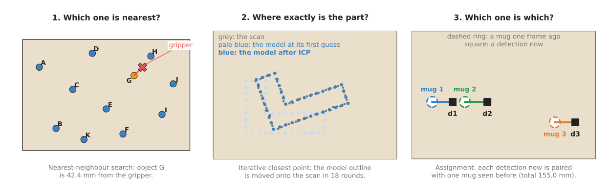
The first panel finds the object nearest to the gripper. The second moves a stored outline of a bracket onto a scan of the real bracket, and the third pairs each mug seen now with a mug seen one frame ago.
All three panels share one idea, because in each of them you measure how far apart two things are with a number called a distance or a cost. Then you look for the smallest distance, or for the set of pairs whose distances add up to the smallest total.
2. The four techniques, in two groups#
Since every one of those jobs comes down to a distance, the chapter has four technique pages, split into two groups.
The most used group holds the three techniques that nearly every robot arm with a camera runs, often many times a second. The other techniques in this book depend on them too.
- Nearest-neighbour search finds, for a query point, the closest point in a set, or the k closest, or all points within a radius. It uses a tree of boxes, called a k-d tree, so that it does not have to measure the distance to every point.
- Iterative closest point (ICP) moves a model of a part onto a scan of the part. It pairs each model point with its nearest scan point, moves the model to fit those pairs, and then repeats those two steps.
- Assignment and matching pairs up two lists, such as the mugs seen one frame ago and the mugs seen now, so that each thing gets at most one partner and the total cost is as small as possible. The Hungarian algorithm does this exactly, while a greedy method does it approximately. ICP's page also has a section on getting a first guess from 3D shape features, for when the part could be turned any way at all.
The also used group holds a technique that is common, but only on some robots: those that must find objects with printing or texture on them from a camera picture.
- Image features and matching finds corners in two pictures, describes the patch round each one as a list of numbers, pairs corners whose lists are alike, and keeps the pairs that agree on one movement of the object. It finds a known flat object, such as a label, and gives the pairs that a 3D pose calculation needs.
The table below compares the four techniques, so read it one row at a time. The row names the technique, while the columns say what goes in, what comes out, and where the technique usually fails.
| Technique | What goes in | What comes out | Where it usually fails |
|---|---|---|---|
| Nearest-neighbour search | a set of points and a query point | the nearest point, the k nearest, or all within a radius | nothing is near enough, or the "distance" does not match what "similar" means |
| Iterative closest point | a model point set, a scan point set, and a first guess of the pose | the rotation and shift that line the model up with the scan | the first guess is too far off, or the part is symmetric |
| Assignment (Hungarian or greedy) | two lists and a cost for every possible pair | a one-to-one pairing, and the things left without a partner | the costs are wrong, or objects are closer together than the measurement error |
| Image features and matching | a stored picture of an object and a camera picture | pairs of matching spots, and the homography or pose that most of them agree on | the object has no texture, or a repeated pattern |
The four build on each other, because ICP runs a nearest-neighbour search in every round. Assignment often uses nearest-neighbour search to fill in its table of costs, or to throw away pairs that are clearly too far apart before it starts. Image feature matching pairs spots with a nearest-neighbour search among their descriptions, and its answer is often the first guess that ICP then makes exact.
3. Why the obvious method is not enough#
Each of those four techniques exists to avoid a simpler method, because for every one of the questions there is an obvious method that is always right: try every possibility. For the nearest point, that means measuring the distance to every point, and for the best pairing it means trying every possible way of pairing the objects up.
Since a table with ten objects needs only ten distance checks, the obvious method is often the right choice when the numbers are small. The trouble is how fast the work grows as the numbers get bigger, and the picture below shows that growth.
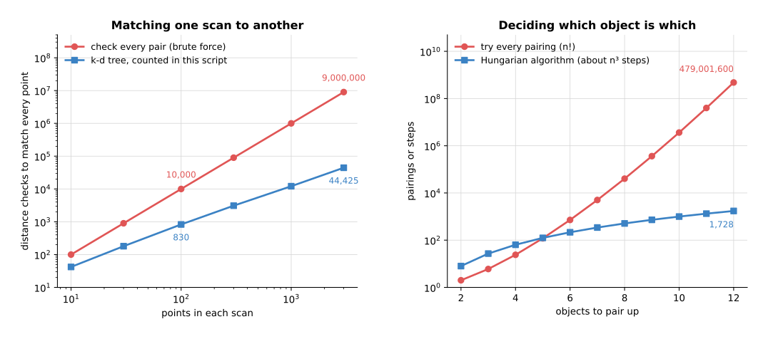
The left panel matches every point of one scan to its nearest point in a second scan of the same size. Checking every pair needs 9,000,000 distance checks for 3,000 points. However, the k-d tree in the diagram script needed 44,425, about 15 per point. The right panel pairs up objects, where trying every pairing of 12 objects means trying 479,001,600 pairings. Instead, the Hungarian algorithm needs roughly 12 × 12 × 12 = 1,728 steps.
A depth camera with a 640 by 480 picture gives up to 307,200 points in each picture, and it gives 30 pictures a second. So checking every pair is not possible on a live camera, and the k-d tree is what makes point cloud work run at all.
4. How this chapter connects to the others#
These techniques are used throughout the book, because searching and matching is the second of the seven families of techniques in it. The map of techniques shows all seven, and the list below says how this chapter connects to the others.
- Geometry and cameras turns pixels and depth into 3D points in the arm's frame, and those points are what this chapter searches. ICP's answer is a rigid transform, the same rotation and shift that chapter explains. Its pose from points page turns the pairs found by image feature matching into a 3D pose.
- Fitting and estimation uses nearest neighbours to find the points on which to fit a plane or a normal. It also supplies the Kalman filter, which predicts where a tracked object should be now, so that assignment can compare detections against the prediction rather than the old position. Its RANSAC throws away the wrong pairs in image feature matching and in ICP's global first guess.
- Image and point cloud processing uses radius search to grow clusters of points into objects, in clustering.
- Decisions and task logic uses the same greedy idea as greedy matching, in greedy algorithms and set cover, and solves larger assignment problems with the optimisation solvers.
Learned models, described in Book 6, do some of the same jobs. For example, a learned tracker can follow objects from frame to frame, as tracking and motion explains, and a learned pose model can find where a known part is without ICP, as keypoints and object pose explains. Even then, the programmed techniques stay in the pipeline, because a learned tracker still usually pairs its boxes with the Hungarian algorithm. A learned pose is also often finished off with a few rounds of ICP to make it more exact.
5. Where to read next#
The pages in this chapter build on one another, so the order below is the one to read them in.
- Start with nearest-neighbour search. The other two pages use it.
- Then read iterative closest point and assignment and matching, in either order.
- Read image features and matching when the arm must find objects from a camera picture rather than a depth scan. It uses nearest-neighbour search, and it helps to have read RANSAC first.
- Book 2's tracking and association goes much deeper into matching objects over time, including how wide to make the gate and what to do when a match fails.
6. Using it in Python#
Section 2 named the four techniques of this chapter and section 3 showed why the obvious method of trying every possibility runs out of time. This section shows the first three of them as the Python calls that already contain them, so that the chapter's shape is clear before you read the pages in detail. After it you should know that none of the three is code you write, and what is left for you is deciding the numbers they take.
Two libraries cover all three. SciPy provides the nearest-neighbour tree and the exact pairing, while Open3D provides iterative closest point.
import numpy as np
from scipy.spatial import KDTree
from scipy.optimize import linear_sum_assignment
import open3d as o3d

# Question 1: which object is nearest the gripper?
objects = np.array([[0.47, 0.21], [0.18, 0.38], [0.33, 0.05], [0.33, 0.18]])
tree = KDTree(objects)
distance, index = tree.query(np.array([0.25, 0.10]), k=1)

# Question 2: exactly where is this part? ICP refines a guess into a pose.
result = o3d.pipelines.registration.registration_icp(
    model_cloud, scan_cloud,
    max_correspondence_distance=0.01,      # metres: pairs further apart are ignored
    init=first_guess_4x4)
T_scan_model = result.transformation

# Question 3: which mug seen now is which mug seen before?
cost = np.linalg.norm(old_positions[:, None, :] - new_positions[None, :, :], axis=2)
old_index, new_index = linear_sum_assignment(cost)
The libraries do the parts that section 3 said were expensive. KDTree builds the
tree of boxes once and then answers each query without touching most of the points,
registration_icp runs the pair-and-move loop until it stops improving, and
linear_sum_assignment finds the pairing with the smallest total cost in roughly
the cube of the number of objects rather than trying every pairing.
What you still write yourself is what surrounds them. You write the cost matrix for the assignment, and that one line of NumPy is where you decide whether "which is which" means position alone or position together with size and colour. You write the first guess that ICP starts from, because ICP only improves a pose and cannot find one. And you write what happens to the things left unpaired, since an object that appeared or disappeared has no partner and the pairing says nothing about it.
What you have to decide or measure is a distance limit in each case, and it is
always a real distance in metres rather than a tuning knob. For the nearest-neighbour
search you decide how far is too far, because the nearest object is not the right
answer when the nearest object is half a metre away. For ICP,
max_correspondence_distance is the pair-rejection distance, which should be a few
times your depth camera's noise. For the assignment you decide the gate, meaning the
distance beyond which a pair is not even considered, and that comes from how far an
object can really move between two pictures. Each of the following pages returns to
its own number in detail.