This page explains thresholding, which is the technique that decides whether a pixel belongs to the thing you are looking for. It makes that decision for every pixel on its own, so no pixel is ever compared with its neighbours.
The page answers four questions, and the first two are about grey pictures: how a threshold turns a picture into a mask, and how the picture itself can choose the limit. The other two questions move on to colour and depth. So the page also asks why robot programs test colour in hue, saturation and value rather than in red, green and blue, and it then shows how the same idea works on a depth picture.
It is for a reader who knows that a picture is a grid of pixels and that each pixel is stored as numbers. Beyond that you need no background in algorithms, because every example here uses a few pixels you can check by hand. Every number on this page came from a real run of the diagram script.
Thresholding is usually the first step of a hand-written perception program, so the overview of this chapter puts it first. It makes the mask that the later steps tidy, trace and group.
Contents#
- The idea in one sentence
- How a brightness threshold works · One limit, one test per pixel · Otsu's method: let the picture choose the limit
- Colour and depth thresholds · Colour in hue, saturation and value · A depth threshold · The steps as pseudocode
- Where it is used on a robot arm
- Where it is useful, and where it is not
- Libraries that provide it
- Why thresholding, and what it costs
- The learned alternative
- Where to read next
- Using it in Python
1. The idea in one sentence#
The whole technique fits into one sentence, and the rest of this page only fills that sentence in. A threshold compares each pixel with a fixed limit, and it writes 1 into a mask where the pixel passes and 0 where it does not.
The limit is called the threshold, and the grid of ones and zeros is called a mask. This mask has one entry for each pixel of the picture. Some libraries store 255 instead of 1 so that the mask can be shown as a black and white picture, but the meaning is the same.
For an everyday example, think of a farmer who sorts eggs by weight. Every egg goes on the scale, and the ones of 63 grams or more go in the "large" box while the rest go in the other box. The farmer never compares one egg with another, because each egg is tested on its own against a single number. A threshold treats pixels in exactly that way.
2. How a brightness threshold works#
One limit, one test per pixel#
That one-sentence idea is easiest to follow on a grey picture, which holds one number per pixel, its brightness. Brightness runs from 0 for black to 255 for white, so a bright object on a dark background is already separated by that one number.
The picture below is a real 6 by 8 grey picture, in which a bright metal part lies on a dark rubber mat. Each square in it shows the brightness number of one pixel.
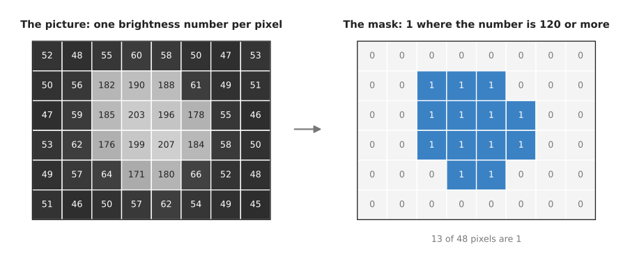
The rule here is "brightness 120 or more", and it works cleanly because the two groups of numbers lie far apart. The mat pixels all fall between 45 and 66, so they all fail, while the part pixels all fall between 171 and 207, so they all pass. So the mask holds 13 ones out of 48 pixels, and those 13 pixels are the part.
Thresholding a whole picture takes only the three steps below.
- Choose the limit, here 120.
- Go through the pixels one at a time.
- If the pixel's number is at the limit or above it, write 1 in the mask. Otherwise, write 0.
Each pixel is tested on its own, and the test never looks at the neighbours. This is why thresholding is so fast, because a computer can test a whole camera picture of 300,000 pixels in well under a millisecond.
Some programs want the dark pixels instead, for example a black part on a white tray. For them the rule becomes "brightness below the limit", while other programs keep a band, with a lower limit and an upper limit. Both are the same idea pointed in a different direction.
Otsu's method: let the picture choose the limit#
The limit of 120 above was chosen by a person, which works only while the light stays the same. Because every number falls when the room gets darker, the part may drop to around 110, and the fixed limit then loses it.
Otsu's method chooses the limit from the picture itself, and it is named after Nobuyuki Otsu, who published it in 1979. It assumes that the picture holds two groups of pixels, a dark group and a bright group. So it tries every possible limit and keeps the one that separates those two groups best.
"Separates best" has an exact meaning, because for each possible limit the method splits the pixels into a dark group and a bright group. It then works out a score for that split:
score = (share of pixels in the dark group)
      × (share of pixels in the bright group)
      × (bright group's average − dark group's average)²
The score is large when the two averages are far apart and when neither group is tiny. So the method simply keeps the limit with the largest score.
Here is a small worked example with 14 pixel values, taken along one line across a mat and a part:
48 52 55 60 63 70 85 110 150 172 180 188 196 201
The value 110 is a pixel on the edge of the part, so it is half mat and half part. This means the method has to decide which of the two groups it belongs to. The table below shows the score for some of the possible splits. Read each row as "put every value up to here in the dark group, and the rest in the bright group".
| Split between | Dark group | Dark average | Bright group | Bright average | Score |
|---|---|---|---|---|---|
| 70 and 85 | 6 values | 58.0 | 8 values | 160.2 | 2,560 |
| 85 and 110 | 7 values | 61.9 | 7 values | 171.0 | 2,978 |
| 110 and 150 | 8 values | 67.9 | 6 values | 181.2 | 3,143 |
| 150 and 172 | 9 values | 77.0 | 5 values | 187.4 | 2,798 |
| 172 and 180 | 10 values | 86.5 | 4 values | 191.2 | 2,239 |
For the best row, the score is 8/14 × 6/14 × (181.2 − 67.9)², which comes out at about 3,143. So Otsu's method puts the edge pixel 110 with the mat, and the six values from 150 upwards with the part. Any limit between 111 and 150 gives that same split.
A real picture has thousands of pixels, so the method works on a histogram instead. A histogram counts how many pixels have each brightness from 0 to 255. This means the method only has to try 255 splits, whatever the size of the picture.
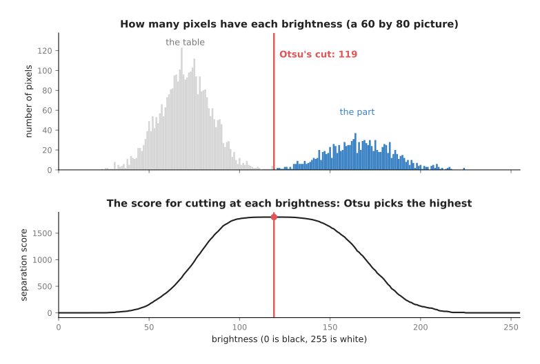
The top panel is the histogram of a 60 by 80 picture that holds a bright part on a dark mat, with some camera noise, and it has two humps. The bottom panel is the score for every possible cut, and the highest score is at 119, in the empty gap between the humps. So 119 is the limit that Otsu's method returns. The score curve is almost flat across that gap, which is good news. This means a small change in the picture moves the limit a little, but the mask hardly changes.
Otsu's method has no number for you to choose, and that is its main strength. Its main weakness is the assumption that there are only two groups. So if the picture holds three groups, for example a dark mat, a grey part and a white label, the method still returns a single limit. This means it may cut through the wrong gap.
3. Colour and depth thresholds#
Colour in hue, saturation and value#
Brightness is enough for a part that is plainly lighter or darker than its background, but many parts are picked out by their colour instead. A colour pixel is usually stored as three numbers, how much red, green and blue it has, and each of them runs from 0 to 255. This way of storing a colour is called RGB.
However, RGB is a poor way to ask "is this pixel red?", because when the light gets weaker all three numbers fall together. A red block might be (200, 40, 40) in the light and (100, 20, 20) in shadow. So a rule such as "red above 150" finds the first and misses the second.
So robot programs convert each pixel to HSV first, which stands for hue, saturation and value. HSV describes the same colour with three more useful numbers.
- Hue says which colour it is, going round a colour circle. In OpenCV, the most used vision library, hue runs from 0 to 179 so that it fits in one byte. Red is near 0, green near 60 and blue near 120.
- Saturation says how strong the colour is, from 0 to 255. Grey, white and black have saturation 0.
- Value says how bright the pixel is, from 0 to 255.
In shadow, a red block keeps its hue and its saturation, and only its value falls. This is exactly why splitting the colour into three numbers helps. The table below shows the numbers for six pixels, as the diagram script computed them on OpenCV's scale. Read each row across to see the pixel, its HSV numbers, and whether each of two rules accepts it.
| Pixel | RGB | Hue | Saturation | Value | "Red above 150" | "Hue 0–10 or 170–179, saturation 100+, value 50+" |
|---|---|---|---|---|---|---|
| red block, lit | (200, 40, 40) | 0 | 204 | 200 | yes | yes |
| red block, in shadow | (100, 20, 20) | 0 | 204 | 100 | no | yes |
| a slightly bluish red | (200, 40, 60) | 176 | 204 | 200 | yes | yes |
| grey table | (120, 120, 120) | 0 | 0 | 120 | no | no |
| white sheet of paper | (235, 235, 235) | 0 | 0 | 235 | yes | no |
| green block | (40, 160, 60) | 65 | 191 | 160 | no | no |
The RGB rule makes two mistakes, because it loses the shadowed red and it accepts the white paper, whose red number is also high. The HSV rule makes neither mistake, since it looks at hue for the colour and at saturation to throw out grey and white. It then looks at value only to throw out pixels that are too dark to judge.
The third row shows a quirk of red, which sits at both ends of the hue circle, just above 0 and just below 179. So a slightly bluish red has hue 176 rather than 2. This means a red rule needs two hue ranges, where every other colour needs only one.
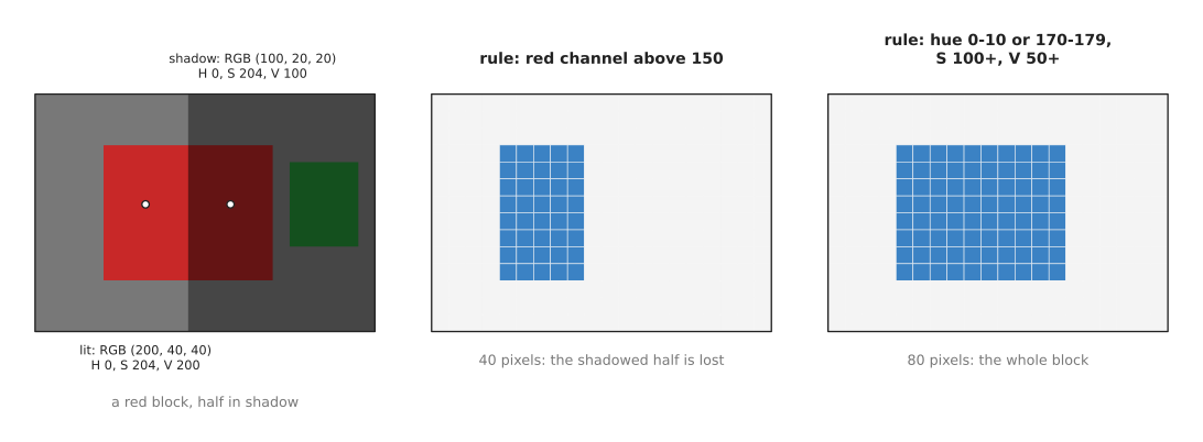
The picture is 14 by 20 pixels, and the red block covers 80 of them. The RGB rule keeps only the 40 lit pixels, while the HSV rule keeps all 80. The green block is also in the shadow, and neither rule keeps it, because both rules are looking for red.
A colour mask has six numbers to choose, a lower and an upper limit for each of hue, saturation and value. So it takes more tuning than a brightness threshold, which has only one. People usually find the six by pointing at the object in a few pictures and reading off its HSV numbers, then leaving some room on each side.
A depth threshold#
Colour separates a part from its background only when the two differ in colour, whereas a depth camera separates them by distance instead. A depth camera gives a depth picture, in which each pixel holds a distance from the camera, often in millimetres. So a depth threshold keeps the pixels whose distance is inside a range.
The most common use is "keep everything nearer than the table". For example, imagine a camera looking straight down at a table 600 millimetres away. Anything standing on that table is nearer than 600, so the rule "distance below 590" keeps every object taller than about 10 millimetres, whatever its colour.
A depth picture has one trap, which is that most cameras write 0 wherever they could not measure. This happens on glass, on shiny metal, on very dark surfaces and along the edges of objects. A reading of 0 would pass the test "below 590", because 0 is below 590, so the rule must also say "above 0".
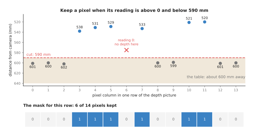
This is one real row of 14 depth pixels, in which the table pixels read 599 to 602 and two objects read between 520 and 538. Pixel 6 reads 0, because the camera saw nothing there. With the rule "above 0 and below 590", the mask keeps 6 of the 14 pixels. Without the "above 0" part it would keep 7, and pixel 6 would count as an object right next to the camera.
However, a missing reading is not always noise to throw away. A patch of zeros shaped like a glass, with the glass clearly visible in the colour picture, is a strong sign of a transparent object. Book 2 uses this in the depth hole, for glass and chrome, where the threshold is simply "reading equals 0".
A fixed limit such as 590 only works if the camera looks straight down at a flat table. That is because a tilted camera sees the table nearer at the top of the picture than at the bottom. So the usual fix is to turn the depth picture into a point cloud, find the table plane with RANSAC, and keep the points higher than 10 millimetres above that plane. This is the same threshold, measured from the table instead of from the camera.
The steps as pseudocode#
The three kinds of threshold described above are written out below as plain steps. This pseudocode does not belong to any programming language.
function brightness_mask(grey, limit):
    mask = a grid the size of grey, filled with 0
    for each pixel p:
        if grey[p] >= limit:
            mask[p] = 1
    return mask

function otsu_limit(grey):
    count = how many pixels have each brightness 0..255
    best_limit = 0, best_score = 0
    for limit from 1 to 255:
        dark   = pixels with brightness below limit
        bright = pixels with brightness at or above limit
        if dark or bright is empty: skip this limit
        score = share(dark) * share(bright) * (average(bright) - average(dark))^2
        if score > best_score:
            best_score = score, best_limit = limit
    return best_limit

function red_mask(colour):
    mask = a grid the size of colour, filled with 0
    for each pixel p:
        h, s, v = convert colour[p] to hue, saturation, value
        red_hue = (h <= 10) or (h >= 170)
        if red_hue and s >= 100 and v >= 50:
            mask[p] = 1
    return mask

function depth_mask(depth, near, far):
    mask = a grid the size of depth, filled with 0
    for each pixel p:
        if depth[p] > 0 and near <= depth[p] < far:
            mask[p] = 1
    return mask
Real libraries do not loop over pixels one by one in slow code. Instead they run the same test on the whole grid at once, in fast compiled code, and the result is the same.
4. Where it is used on a robot arm#
Now that all three kinds of threshold are on the table, it is worth seeing where they actually turn up. Thresholding appears in almost every hand-written perception program on an arm, and the list below gives some concrete places.
- A coloured part is found with a colour mask, so a red block, a blue bin or a green marker on a table is picked out by an HSV mask. The middle of the mask, together with the depth at that pixel, gives the point the arm reaches for, and Book 2 runs this end to end in finding it by colour.
- Anything that stands on the table is found with a depth threshold, because a threshold measured from the table plane keeps every object whatever its colour. This is the first step of the classic "remove the plane, then cluster" recipe, described in Book 2 under point clouds: remove the plane, then cluster.
- The point cloud is cropped to the workspace by a box-shaped threshold on x, y and z, which keeps only the points inside the arm's reach. It throws away the floor, the walls and the robot's own base, and so it makes every later step faster.
- A depth threshold checks that the gripper holds something, because a wrist camera looks between the fingers and the program counts the depth pixels nearer than the fingertips inside a small window. If that count is above a limit, then something is in the gripper.
- Otsu's method suits parts on a backlit tray, since a light box under the tray makes every part a dark shadow on a white background. Otsu's method then finds the limit on its own, even as the lamp ages and dims.
- A depth threshold notices a person entering the cell, because a fixed overhead depth camera watches the cell all the time. If more than a set number of pixels become nearer than the empty floor, then something has entered, and the arm slows down or stops.
- A threshold turns a learned model's scores into a mask, because a segmentation model gives each pixel a number from 0 to 1 saying how sure it is that the pixel belongs to an object. A threshold, often 0.5, turns that into a mask, so even a learned pipeline ends in a threshold.
5. Where it is useful, and where it is not#
All of those uses share one condition, which is that a single simple number separates the object from everything else. That number is its brightness, its colour or its height. So thresholding fails whenever no such number exists, and the table below lists the common failures. Read each row as: this goes wrong, this is what you see, and this is what people use instead.
| What goes wrong | The sign you would see | What people use instead |
|---|---|---|
| The light changes, for example daylight through a window | The mask shrinks or grows during the day; the part is lost in the evening | HSV instead of RGB; Otsu's method; a lamp you control; a depth threshold |
| Uneven light, bright on one side of the table and dark on the other | Otsu's limit is right on one side and wrong on the other | An adaptive threshold, which picks a separate limit for each small area of the picture |
| The object is the same colour as the background, such as a white mug on a white table | The mask is empty, or it covers the whole table | A depth threshold, or a segmentation model |
| Two objects of the same colour touch | One patch in the mask where there should be two | The distance transform and watershed, or 3D clustering |
| A shiny highlight on the object | A hole in the middle of the mask | Closing to fill the hole |
| Camera noise near the limit | Single specks scattered across the mask | Opening, or a small blur before the threshold |
| Glass, mirrors and polished metal | Zeros in the depth picture; colour taken from whatever is behind | Treat the zeros as a signal, or use a learned depth model such as depth from pictures |
| Many kinds of object, each a different colour | One mask per colour, and a new rule every time a new part arrives | A trained object detector |
Book 2 lists the same failures from the other side in when colour stops working.
6. Libraries that provide it#
Because those failures and their fixes are so well known, they are already built into the standard libraries. So you rarely write a threshold yourself, apart from the one-line comparison. The table below lists well-known libraries that provide thresholds out of the box. Read each row as the library, the languages you can call it from, the function or class to look for, and a note on what to watch.
| Library | Languages | Function or class | Note |
|---|---|---|---|
| OpenCV | C++, Python | cv2.threshold with THRESH_BINARY; add THRESH_OTSU for Otsu's method | Otsu's method needs an 8-bit grey picture |
| OpenCV | C++, Python | cv2.adaptiveThreshold | A separate limit for each small area, for uneven light |
| OpenCV | C++, Python | cv2.cvtColor with COLOR_BGR2HSV, then cv2.inRange | OpenCV reads pictures as blue, green, red; hue runs 0 to 179 |
| scikit-image | Python | skimage.filters.threshold_otsu, skimage.color.rgb2hsv | Its HSV numbers run from 0 to 1, not 0 to 179 and 0 to 255 |
| NumPy | Python | the comparison operators, such as grey >= 120, and np.logical_and | A threshold is one line; the result is an array of true and false |
| Open3D | C++, Python | PointCloud.crop with an AxisAlignedBoundingBox | A box-shaped threshold on a point cloud |
| PCL (Point Cloud Library) | C++ | pcl::PassThrough | Keeps points whose x, y or z is inside a range |
When you copy HSV limits from one library to another, check the scale first. This matters because a hue of 0.5 in scikit-image is a hue of 90 in OpenCV.
7. Why thresholding, and what it costs#
With the libraries in hand, the remaining question is when to reach for thresholding at all. So this section answers the four standard questions: what it is, what it does for you, why it rather than the obvious alternative, and what it costs.
It is a test applied to each pixel on its own, against a fixed limit or a range. This turns a picture into a mask of the pixels that might be the object. It runs in well under a millisecond, needs no training and no graphics card, and gives the same answer every time for the same picture. So when it goes wrong, you can find out why by reading one pixel's numbers.
The obvious alternative is a learned segmentation model, and Section 8 says when each one is the better choice.
The second obvious alternative is to skip the mask and go straight to 3D clustering. But clustering needs a depth camera, and it still needs a threshold first to remove the table. So in practice the two are used together rather than one instead of the other.
Against all that, you must choose the limits, and a colour mask has six of them, so there is real tuning work before anything runs. Because those limits are tied to the light, the camera and the objects, they need checking again whenever one of those three changes. A threshold also only says "might be the object". So it cannot tell two touching objects apart, and it cannot say what an object is.
8. The learned alternative#
That first alternative is worth a closer look, because Book 6 has two kinds of model that do this same job. A segmentation model marks the pixels of each object without any hand-set limits, and an object detector puts a named box round each object. A model wins when you cannot control the scene, because it handles mixed colours, clutter and changing light much better. It also copes with many kinds of part without a new rule for each one. However, a threshold still wins when the object has a property that nothing else in the scene shares. That property may be a colour you chose, a height above a known table, or a brightness against a backlit tray. In a robot cell you often control these things, so a threshold is the right answer more often than its simplicity suggests.
9. Where to read next#
- The next page is morphology and the distance transform, which removes the specks and fills the holes that a threshold leaves behind.
- Clustering turns a mask into separate objects, and does the same for a point cloud.
- RANSAC finds the table plane that a height threshold is measured from.
- The pinhole camera model turns the middle of a mask into a 3D point.
- Book 2 has real code for an HSV mask in finding an object in a picture, and a summary of colour ranges in methods you write yourself.
10. Using it in Python#
Section 2 explained the one test per pixel, section 3 explained the colour and depth versions, and section 6 listed the OpenCV calls that do both. This section puts those calls in a program. After it you will be able to turn a picture into a mask in three lines, and you will know which of the numbers in those lines you have to measure in your own workcell.
The program below makes two masks from the same picture. The first is the brightness threshold with Otsu's method, where the picture chooses the limit itself. The second is the colour mask from section 3, which converts to hue, saturation and value first and then keeps the pixels inside a range. Both come from OpenCV, which reads pictures as blue, green, red rather than red, green, blue.
import cv2
import numpy as np

picture = cv2.imread("scene.png")
grey = cv2.cvtColor(picture, cv2.COLOR_BGR2GRAY)

# A brightness limit chosen by Otsu's method.  The limit it picked comes back
# as `limit`; the 0 passed in is ignored when THRESH_OTSU is used.
limit, bright = cv2.threshold(grey, 0, 255, cv2.THRESH_BINARY + cv2.THRESH_OTSU)

# A colour mask: hue 40 to 80 is green in OpenCV, whose hue runs 0 to 179.
hsv = cv2.cvtColor(picture, cv2.COLOR_BGR2HSV)
mask = cv2.inRange(hsv, np.array([40, 80, 40]), np.array([80, 255, 255]))

# A depth threshold is the same idea on a depth picture, in metres.
depth = np.load("depth.npy")
above_table = (depth > 0.30) & (depth < 0.70)
On a made-up 320 by 240 picture of two green blocks on a grey table, Otsu's method picks a limit of 138 and marks 68457 pixels as bright, which is the table and not the blocks, because the table is the brighter of the two. The colour mask keeps 8152 pixels, which is the two blocks. That difference is the whole argument of section 3: brightness alone cannot tell a green block from a grey table of similar brightness, and colour can.
OpenCV does the per-pixel comparison and, for Otsu's method, the search for the
limit as well. cv2.threshold returns two values, and the first is the limit it
chose, which is worth printing because a limit that jumps between pictures tells
you the lighting is changing. cv2.inRange tests all three channels at once and
returns a mask of 0 and 255, and the & on the depth arrays is NumPy doing the
same thing on true and false values. The last line shows why the depth version
needs no library at all: a comparison on a NumPy array already is a threshold.
What you still have to write is what happens to the mask. A mask is not an answer, because it is a picture of true and false values, and the arm needs a position. The morphology page cleans the mask and the clustering page turns it into separate objects with centres, and those two steps almost always follow this one.
What you have to decide or measure is the limits, and this is the part that decides whether the mask works tomorrow as well as today. The hue range of 40 to 80 above is a claim about your lighting and your camera, so you measure it by opening real pictures of your own workcell and reading the hue values off the pixels you want to keep. The saturation floor of 80 and the value floor of 40 matter just as much, because a very pale or very dark pixel has an unreliable hue, and leaving those floors at 0 is the usual reason a colour mask picks up half the room. For the depth mask you decide 0.30 and 0.70 metres, which are distances in your own camera's frame, so moving the camera changes them. Otsu's method looks like it removes the decision, but it only moves it: it assumes the picture has two groups of brightnesses, and section 2 explains what it returns when that assumption is false.