This page explains how a robot turns many depth pictures into one 3D map of the space round it. It answers five questions, and the first four of them follow the order in which the map is built. How is space cut into small cubes, and how is each cube marked as free, occupied or not yet seen? How does a program combine many noisy depth readings of the same cube into one answer? Why do most maps store their cubes in a tree instead of a plain grid? What are the truncated signed distance function (TSDF) and the Euclidean signed distance field (ESDF), and why do planners like them? And which libraries do this, and which of them are used most?
It is for a reader who knows what a depth picture and a point cloud are. While a depth picture holds one distance for each pixel, a point cloud is the list of 3D points you get by turning each depth pixel into a point. That step is explained on the pinhole camera model page, and it also helps to have read about voxel downsampling, which cuts space into the same small cubes this page uses.
One depth picture only shows the surfaces in front of the camera at one moment. But a robot arm needs more than that, because it has to remember the shelf behind it after it has turned away. It also has to know that the space under its gripper is empty, and to know which space it has never seen at all. A volumetric map holds all of this, and "volumetric" means that it describes the space itself, cube by cube, and not only the surfaces.
Contents#
- The idea in one sentence
- How it works · Step 1: cut space into voxels · Step 2: cast a ray for each depth pixel · Step 3: combine readings with log-odds · Step 4: store the map in a tree · Step 5: the truncated signed distance function · Step 6: the distance field that planners read · The steps as pseudocode
- Where it is used on a robot arm
- Where it is useful, and where it is not
- Libraries that provide it
- Why a volumetric map, and what it costs
- The learned alternative
- Where to read next
- Using it in Python
1. The idea in one sentence#
A volumetric map cuts space into small cubes and, for every depth reading, marks the cubes the camera saw through as more likely free and the cube where the reading ended as more likely occupied, so that many readings add up to one steady answer.
For example, you walk into a dark room with a torch. Each time you shine it, the beam passes through empty air and stops on a wall or a chair. This means you learn two things from each beam: the air along the beam is empty, and something solid stands where the beam stopped. But corners you never shine the torch at stay unknown. After a few minutes of shining the torch round, you have a good picture of the room in your head, even though no single beam showed you much. So a volumetric map does the same with the thousands of beams in each depth picture.
2. How it works#
The map described in the last section is built in six steps. Steps 1 to 4 build an occupancy map, which says for each cube whether it is free, occupied or unknown. Then steps 5 and 6 build two other kinds of map from the same readings. While one of them gives a smooth surface, the other gives the distance to the nearest obstacle, which is what many planners read.
All the pictures on this page show a slice of a table seen from above, 64 cm by 64 cm, cut into cells of 1 cm. A real map is 3D, with cubes instead of squares, but every step works the same way. The table holds a box, a round tin and, at the back, a wall.
Step 1: cut space into voxels#
A voxel, short for "volume pixel", is one small cube of space. That is why the map cuts the robot's work space into voxels of equal size and keeps a few numbers for each one. The size of a voxel is called the resolution, and for a table-top arm it is usually 1 to 2 cm. Because a smaller voxel shows more detail, it also needs more memory and more time.
But a plain grid of voxels grows fast, because a cube of space 1 m on each side, cut into 1 cm voxels, has 100 × 100 × 100 = 1,000,000 voxels. So step 4 shows how a tree cuts that number down.
Step 2: cast a ray for each depth pixel#
Each depth pixel says "along this line from the camera, the first surface is at this distance". So the program follows that line, called a ray, from the camera to the measured point. This is called ray casting, and along the way it collects two kinds of voxel:
- every voxel the ray passes through before the end. The camera saw through them, so they are evidence for free. This is called a miss.
- the voxel where the ray ends. Something is there, so it is evidence for occupied. This is called a hit.
But voxels behind the end point get nothing, because the camera cannot see behind a surface, so they stay unknown. Unknown is not the same as free, because the space behind a box might hold another object.
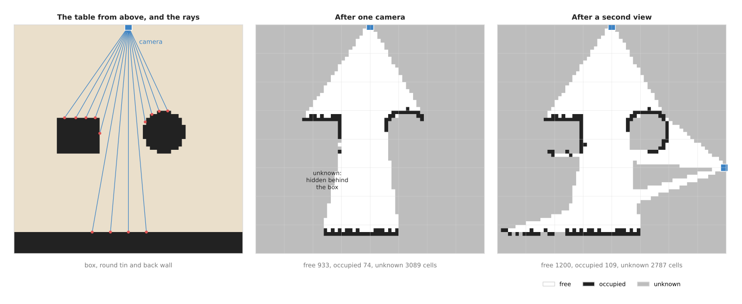
The left panel shows the real scene and every tenth ray of the camera. The camera has a 70° view and 141 rays, and each ray's reading has a small random error of about 3 mm. While the middle panel is the map after three pictures from that camera, the right panel adds three pictures from a second camera position on the right.
After the first camera, 933 cells are free, 74 are occupied and 3,089 are unknown. Most of the map is unknown, because the camera only sees a wedge of the table, and the areas behind the box and the tin are hidden. The second view sees round the tin and along the right of the table. As a result, free cells rise to 1,200, occupied cells to 109, and unknown cells fall to 2,787. But the inside of the box and the tin stays unknown in both maps, because no camera can see inside a solid object.
However, the occupied cells are not perfect lines: where a ray grazes a surface at a shallow angle, the small reading error puts its end in the cell next door. Step 3 is how the map copes with that error.
A real program steps along each ray with a method that visits exactly the voxels the ray crosses, one after another. The usual one was published by John Amanatides and Andrew Woo in 1987.
Step 3: combine readings with log-odds#
A single reading can be wrong, because a depth camera makes stray points at the edges of objects, and a hand can pass through the view for one frame. So a map does not say "free" or "occupied" after one reading. Instead it keeps, for each voxel, a probability: a number from 0 to 1 that says how likely the voxel is to be occupied. Every voxel starts at 0.5, which means "no idea".
Then each new reading changes that probability a little. The most common library, OctoMap, uses these default values. While a hit means the voxel is occupied with probability 0.7, a miss means it is occupied with probability only 0.4. This means that after one hit, a voxel's probability is 0.7, and after two hits it is 0.845. After one hit and then one miss it is 0.609.
But multiplying probabilities together is awkward and slow, so the map stores each voxel's value as a log-odds number instead. The odds of a voxel are its probability of being occupied divided by its probability of being free, and the log-odds is the natural logarithm of the odds. This is useful because, to combine a new reading, you simply add a fixed number. The table below gives that number for the two kinds of reading, so read a row as one kind of reading, the probability it stands for, and the amount it adds to the voxel's log-odds.
| reading | probability it stands for | number added to the log-odds |
|---|---|---|
| hit | 0.7 | +0.847 |
| miss | 0.4 | −0.405 |
So every hit adds 0.847 to the voxel's log-odds, and every miss subtracts 0.405. A log-odds of 0 means a probability of 0.5. Therefore a positive log-odds means "probably occupied", and a negative one means "probably free". A voxel that was never touched by any ray stays at exactly 0, which marks it as unknown.
There is one more rule, because the log-odds is clamped: it is not allowed to go above +3.511, which is a probability of 0.971, or below −2.0, which is a probability of 0.1192. Without this cap, a voxel that was seen many times would become so certain that it could hardly change again. The picture below shows why that cap matters.
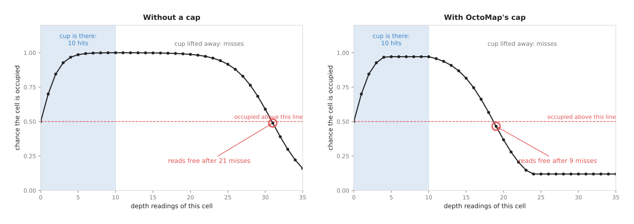
Because a cup stands on the table for 10 depth pictures, its voxel gets 10 hits. Then the arm lifts it away, and every following picture gives the voxel a miss.
Without a cap, 10 hits give a log-odds of 8.47, a probability of 0.9998. Then it takes 21 misses before the voxel reads free again. At 30 pictures a second, the map would show a ghost cup for most of a second after the cup has gone. But with the cap, the log-odds stops at 3.511 after the fifth hit, and it then takes only 9 misses to read free. In other words, the cap costs a little certainty and buys a map that keeps up with a changing table.
Step 4: store the map in a tree#
Most of a work space is either empty air or unknown. But a plain grid spends the same memory on a big block of empty air as on the edge of an object. So a tree avoids that waste.
An octree is a tree of cubes, and the whole work space starts as one big cube. If everything inside it is the same, it stays one cube. But if not, it is cut into 8 equal smaller cubes, and each of those is checked in the same way, down to the smallest voxel size. In 2D, the same idea cuts a square into 4 smaller squares, and then the tree is called a quadtree.
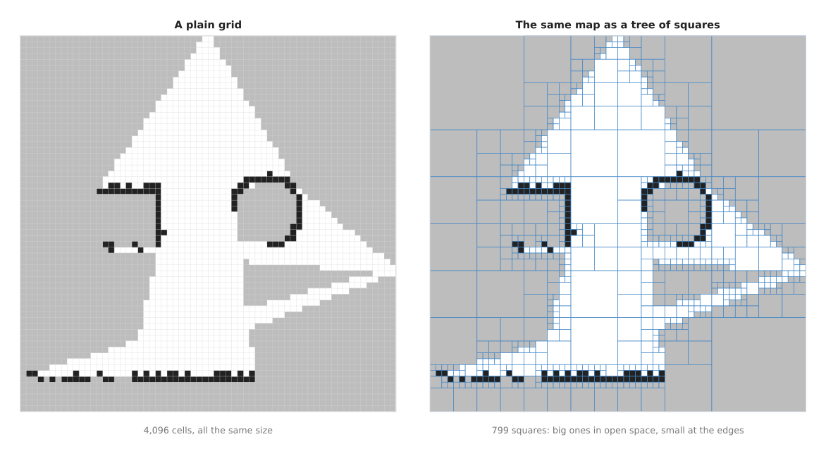
The left panel is the two-view map from step 2 as a plain grid of 64 × 64 = 4,096 cells. While the right panel is the same map as a quadtree, it needs only 799 squares. Of these, 556 are single cells at the edges of objects and of the camera's view, 157 are 2 × 2 blocks, 66 are 4 × 4, 17 are 8 × 8 and 3 are 16 × 16. Because the big squares hold open air and unknown space, the map says exactly the same thing with a fifth of the pieces.
In 3D the saving is much larger, because a big cube holds 8 times as many voxels at each level, not 4. This is why OctoMap, the most used occupancy map, is an octree. It has a second benefit as well, because a program can ask the map at a coarser level, such as "is anything in this 8 cm cube?", with one look.
Step 5: the truncated signed distance function#
An occupancy map is good for "is this space free?". But it is poor at showing the exact shape of a surface, because each voxel is only "in" or "out". So a signed distance function stores something more precise: for each voxel it stores the distance from the voxel's centre to the nearest surface. The sign says which side the voxel is on: positive in front of the surface, in free space, and negative behind it, inside the object. This means the surface itself is where the value crosses zero.
A truncated signed distance function (TSDF) only keeps the exact value close to the surface. So values further than a chosen truncation distance are cut off at that distance. Many libraries go further and only visit the voxels inside this thin band. Because the camera knows nothing about voxels far behind a surface, those voxels are not updated at all. So keeping only a thin layer round each surface saves work, and it stops one side of a thin object from wiping out the other.
Each new depth picture updates the TSDF by a weighted average. For each voxel near the measured surface, the program works out the signed distance from this reading, then mixes it into the stored value. For example, take one camera ray, with 1 cm voxels and a truncation distance of 3 cm. A surface stands 50.0 cm from the camera, and three depth readings measure it at 50.4, 49.7 and 50.2 cm.
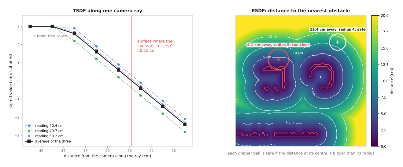
While the left panel shows the TSDF along the ray, the right panel is the distance field of step 6.
Take the voxel whose centre is at 49.5 cm. Because the first reading says the surface is at 50.4, this voxel is 50.4 − 49.5 = 0.9 cm in front of it. The other two readings give 0.2 and 0.7, so the average of the three is 0.6. The next voxel, at 50.5 cm, gets −0.1, −0.8 and −0.3, which average to −0.4. This means the value crosses zero between these two voxels, and a straight line between them crosses zero at 49.5 + 0.6 / (0.6 + 0.4) = 50.10 cm. That is exactly the average of the three readings, and within 1 mm of the true surface. Because the voxels at 53.5 and 54.5 cm are more than 3 cm behind every reading, they are not updated.
This is how a TSDF turns many noisy depth pictures into one smooth surface, finer than its own voxels. A program then pulls a triangle mesh out of the zero crossing with a method called marching cubes. The method became well known through KinectFusion, published in 2011, which built live 3D models this way from a moving depth camera. The TSDF itself goes back to Brian Curless and Marc Levoy in 1996.
Step 6: the distance field that planners read#
A planner does not need to know what an obstacle looks like. Instead it needs to know how far each point of the arm is from the nearest obstacle. So a Euclidean signed distance field (ESDF) stores exactly that for every voxel: the straight-line distance from the voxel to the nearest occupied voxel, which is negative inside obstacles.
This is the same idea as the distance transform, which measures how far each pixel of a mask is from the nearest edge. An ESDF does it in 3D, for the free space outside the obstacles. Libraries build it from the TSDF or the occupancy map by spreading a wave out from the surfaces, one layer of voxels at a time.
The right panel of the picture above shows the ESDF of the two-view map, with lines at 5, 10 and 15 cm from the nearest obstacle. In this picture only the occupied cells count as obstacles. A planner models the arm as a set of balls. This means a ball is clear of every obstacle when the ESDF at its centre is bigger than its radius, and that is one look-up per ball, however many obstacles there are.
The picture checks two balls that stand for parts of the gripper. The ball at (50, 13) cm has a radius of 4 cm, and the ESDF at its centre is 12.4 cm, so it is clear by 8.4 cm. But the ball at (21, 21.5) cm has a radius of 5 cm, and the ESDF at its centre is only 4.1 cm. This means it overlaps the box by 0.9 cm, and the planner rejects that pose.
An ESDF also says which way is "away from the obstacle": the direction in which the distance grows fastest. So optimisation planners such as CHOMP use that direction to push a path away from obstacles, as the trajectory optimisation page explains.
The steps as pseudocode#
The six steps above come together in the pseudocode below. It has one function for the occupancy update, one for reading a voxel's state, one for the TSDF and one for the ESDF look-up.
function update_occupancy(map, camera_position, depth_points):
    for each measured point q in depth_points:
        cells = the voxels on the ray from camera_position to q
        for each voxel v in cells, except the last:
            map.log_odds[v] = max(L_MIN, map.log_odds[v] + L_MISS)    # seen through: free
        v = the voxel that holds q
        map.log_odds[v] = min(L_MAX, map.log_odds[v] + L_HIT)         # seen: occupied

function state(map, v):
    if v was never updated: return UNKNOWN
    if map.log_odds[v] > 0:  return OCCUPIED
    else:                    return FREE

function update_tsdf(tsdf, weight, camera_position, depth_points, trunc):
    for each measured point q in depth_points:
        for each voxel v on the ray, up to trunc behind q:              # nothing further behind
            sd = distance(camera, q) - distance(camera, centre of v)   # + in front, - behind
            sd = min(sd, trunc)
            tsdf[v]   = (tsdf[v] * weight[v] + sd) / (weight[v] + 1)   # running average
            weight[v] = weight[v] + 1

function is_clear(esdf, arm_balls):
    for each ball (centre, radius) in arm_balls:
        if esdf.look_up(centre) <= radius: return false
    return true
With OctoMap's defaults, L_HIT is +0.847, L_MISS is −0.405, L_MIN is −2.0
and L_MAX is +3.511.
3. Where it is used on a robot arm#
The six steps above describe the map on its own, so this section shows where it sits in a real arm's software. A volumetric map sits between the depth camera and the parts of the program that must not hit anything, and the places below are the common ones.
- Avoiding obstacles nobody put in the model. A planning program knows the shape of the arm and of the fixed table, but it does not know about a toolbox someone left on the table. That is why MoveIt, the most used planning framework for arms, builds an OctoMap from the depth camera for exactly this, and its planners then treat every occupied voxel as an obstacle. Book 3 describes this in the planning scene.
- Remembering what the camera cannot see now. A camera on the wrist looks wherever the gripper points, so when the arm turns to a shelf, the table behind it leaves the view. The map keeps the table's voxels, so the planner still avoids them.
- Removing the arm from its own map. The arm is often in the camera's view, and its own points would fill the map with false obstacles right where the arm wants to move. So MoveIt removes every point that lies on the arm's known shape, plus a small margin, before it updates the map.
- Planning fast with a distance field. GPU planners such as NVIDIA's cuMotion can read an ESDF built by nvblox, and optimisation planners use its distance and direction at every waypoint.
- Scanning an object before grasping it. A camera on the wrist takes pictures from several sides of a part, and a TSDF fuses them into one closed mesh. A grasp planner then works on the whole shape, not only the side one picture showed.
- Choosing where to look next. Unknown voxels show where the robot has not looked, so a program can pick the next camera pose that would turn the most unknown voxels into known ones. Book 2 covers this in choosing where to look, and this book in visibility and next best view.
- Checking whether a space is empty. Before placing a part in a bin, the arm asks the map whether the voxels where the part will go are free, and not only "not occupied", because an unknown voxel means "look first".
But a volumetric map is not a measuring tool. Book 2 warns about this in packages for measuring: an occupancy map with 1 or 2 cm voxels is the model of what the arm must not hit, not the model of the part it is about to grasp. Instead the part itself is measured on the point cloud, with the methods on the clustering and RANSAC pages.
4. Where it is useful, and where it is not#
The places in the last section all assume the same conditions. A volumetric map works best when the camera's pose is known well, the depth is good, and the scene changes slowly compared with the camera's frame rate. But it fails in a few common ways, and the table below lists them.
Read each row as: this is what goes wrong, this is what you would see, and this is what people do instead.
| what goes wrong | the sign you would see | what people do instead |
|---|---|---|
| The camera's pose is wrong, from a bad hand-eye calibration or a late joint reading | Walls and objects appear twice, or smeared; free space eats into real obstacles | Recalibrate; use the joint angles from the same moment as the picture; slow the arm while mapping |
| The voxels are too big | The planner refuses gaps the gripper could pass through; thin rods vanish or grow fat | A smaller voxel near the work area; a separate precise model for the part being grasped |
| The voxels are too small | The map update is slow, and memory grows | A larger voxel; a GPU library such as nvblox; update the map at a lower rate than the camera |
| Glass, shiny metal or black foam | Missing hits, so a real obstacle reads as free or unknown | Treat unknown space as blocked near the arm; add the object as a known shape; see Book 2's the depth hole |
| Objects that move quickly, such as a person's hand | Ghost obstacles that stay after the hand has gone, or a hand that is missed | Clamping, as in step 3; clear the map before each plan; a separate safety sensor for people |
| The arm's own body is not fully removed | A cloud of false voxels round the gripper, and the planner reports that the start pose is in collision | A larger removal margin; check the arm model and the camera's pose |
| Unknown space treated as free | The planner sends the arm into space no camera has seen | Mark unknown voxels near the path as obstacles, or look there first |
5. Libraries that provide it#
None of the six steps has to be written from scratch, because four libraries do most of this work for robot arms. Read the table below as: this library, used from these languages, does this, and this is where it is used.
| library | languages | what it builds | where it is used most |
|---|---|---|---|
| OctoMap | C++, with ROS wrappers | A log-odds occupancy octree, with the clamping of step 3. The main class is octomap::OcTree, with insertPointCloud and castRay. | The most used occupancy map for arms, because MoveIt uses it. MoveIt's occupancy map monitor builds it from a point cloud or a depth picture. The library is BSD; its octovis viewer is GPL. |
| Open3D | Python, C++ | A TSDF, with open3d.pipelines.integration.ScalableTSDFVolume and the newer open3d.t.geometry.VoxelBlockGrid, and a mesh from its zero crossing. | The most used way to fuse depth pictures into a mesh in Python: scanning an object, or a scene for a digital twin. It does not build an ESDF for planning. |
| nvblox | C++ on an NVIDIA graphics card, Python, ROS 2 through Isaac ROS | A TSDF, an ESDF and a mesh, updated on the graphics card many times a second. | NVIDIA's robot stack: its planner cuMotion and its cuRobo library can use its maps. It needs an NVIDIA card. |
| voxblox | C++, ROS 1 | A TSDF, then an ESDF built from it step by step as new pictures arrive. | Research, and flying robots, where it began. It is written for ROS 1 and there is no official ROS 2 version, so new arm projects rarely start with it. |
In plain words: if you use MoveIt, you already use OctoMap, and it is the one to learn first. But if you want a clean 3D model of an object or a scene from a handful of depth pictures, use Open3D's TSDF. And if you have an NVIDIA card and a planner that reads a distance field, use nvblox. Since voxblox is the older CPU version of the same idea as nvblox, you will meet it mainly in papers.
In MoveIt, the map is set up in a file usually called sensors_3d.yaml. It names
the sensor plugin, such as occupancy_map_monitor/PointCloudOctomapUpdater, the
topic to read, the maximum range, and the margin used to remove the arm's own
body. But the voxel size is a separate setting, octomap_resolution.
6. Why a volumetric map, and what it costs#
The libraries in the last section make a volumetric map easy to build. So this section asks whether you need one at all. It answers the four questions for this technique: what it is, what it does for you, why it rather than the obvious alternative, and what it costs.
A volumetric map is a grid of small cubes, often stored as a tree, in which each cube holds either a probability of being occupied or a distance to the nearest surface. Then every depth picture updates it by casting rays from the camera.
What it does for you is give one steady answer, built from many noisy pictures, to three questions: is this space free, is it occupied, or has the robot not looked there yet? It also remembers space the camera no longer sees. And, with a distance field, it tells a planner how far every point is from the nearest obstacle in one look-up.
The obvious alternative is to skip the map and use the latest point cloud directly as the obstacle. That is simpler and has no delay, and some collision checkers can take a point cloud. But a single cloud has holes, stray points and no memory, so it says nothing about the space behind objects, or about space that left the view a second ago. And it cannot tell "free" from "not seen", which is the difference between safe and unsafe. So choose the raw cloud when the scene is fully in view and nothing is hidden. But choose a map when the camera moves, when parts of the scene are hidden, or when the robot must be sure a space is empty.
A second alternative is a learned model that fills in the 3D shape, and Section 7 compares the two.
The costs of a volumetric map come in several parts. Because the map is only as good as the camera's pose, it needs a good calibration and exact timing. You must also choose the voxel size, which is a trade between detail, speed and memory. Since a 3D map at 1 cm has up to a million voxels per cubic metre, updating it at the camera's full rate takes real computing time. This is why nvblox moves that work to the graphics card. Moving objects leave ghosts unless the map is clamped or cleared. And the map is coarse by design, because it tells the arm what not to hit, not the exact shape of what to grasp.
7. The learned alternative#
Section 6 named a learned model as the second alternative, so this section says what those models can and cannot do. No model in Book 6 replaces the map as the record of free, occupied and unseen space, but three kinds of model help it. For example, a shape completion model guesses the hidden back of an object from one view, where the map keeps it as unknown. Then scene reconstruction builds a 3D scene from colour photos, so it sees glass and shiny surfaces that leave holes in a depth map. But it takes seconds to minutes, and the scene must stay still. A learned collision checker, from learned motion planners, gives a fast distance to obstacles like an ESDF. But it is least reliable near the edge of an obstacle. So for collision avoidance the map still wins, because it never guesses: it keeps unseen space as unknown, and that honesty is what keeps the arm safe. In practice the map and the models are often used together.
8. Where to read next#
- Clustering covers voxel downsampling, the same grid of cubes used to thin a point cloud.
- Morphology and the distance transform explains the 2D distance transform that an ESDF extends to 3D.
- Sampling-based planning explains the collision checks that read this map, and trajectory optimisation uses the distance field to push a path away from obstacles.
- Visibility and next best view uses the unknown voxels to choose where the camera should look.
- Book 2's choosing where to look casts rays in 3D to test what a camera can see.
- The chapter overview compares all the techniques in this chapter.
- The diagrams on this page are drawn by
docs/diagrams/image_processing_3.py. Every number on the page comes from the functions in that script; run it with--numbersto print them.
9. Using it in Python#
Section 2 worked through the six steps from voxels to a distance field, and section 5 said that four libraries already do most of them. Those four are not equally reachable from Python, so this section shows the one that is. After it you will be able to fuse depth pictures into a mesh from a Python script, and you will know why the map a planner reads is not built this way.
The program below is the truncated signed distance function, or TSDF, from step 5, built with Open3D. It takes a colour picture and a depth picture together with the camera's pose, adds them into the volume, and pulls a mesh out of the zero crossing.
import numpy as np
import open3d as o3d

width, height, focal = 640, 480, 600.0
camera = o3d.camera.PinholeCameraIntrinsic(width, height, focal, focal,
                                           width / 2 - 0.5, height / 2 - 0.5)

volume = o3d.pipelines.integration.UniformTSDFVolume(
    length=0.30,          # the side of the box the map covers, in metres
    resolution=128,       # voxels along that side, so 0.30 / 128 is the voxel size
    sdf_trunc=0.02,       # how far either side of the surface distances are kept
    color_type=o3d.pipelines.integration.TSDFVolumeColorType.RGB8,
    origin=np.array([-0.15, -0.15, 0.35]))    # the box's corner, in world metres

for colour_file, depth_file, pose in pictures:
    rgbd = o3d.geometry.RGBDImage.create_from_color_and_depth(
        o3d.io.read_image(colour_file), o3d.io.read_image(depth_file),
        depth_scale=1000.0,     # the depth picture is in millimetres
        depth_trunc=1.0,        # ignore anything further than 1 metre
        convert_rgb_to_intensity=False)
    volume.integrate(rgbd, camera, np.linalg.inv(pose))   # pose is camera to world

mesh = volume.extract_triangle_mesh()
mesh.compute_vertex_normals()
On a made-up depth picture of a 50 mm ball half a metre in front of the camera,
one call to integrate fills 20724 voxels and extract_triangle_mesh returns
3180 vertices and 5778 triangles. The voxel size is 0.30 divided by 128, which
is 2.34 mm, and that is the finest detail the mesh can carry however many
pictures you add.
Open3D does steps 1, 2, 3 and 5 for you. It cuts the box into voxels, walks
along the ray for every depth pixel, combines the new reading with what each
voxel already held, and runs the marching cubes step that turns the stored
distances into triangles. UniformTSDFVolume holds a fixed box, which suits one
object on a turntable, and ScalableTSDFVolume takes the same integrate call
but allocates blocks as they are needed, which suits a whole scene whose extent
you do not know in advance.
What you still have to write, and this is the honest answer the section 5 table
implies, is the map that a planner reads. Open3D builds a TSDF and a mesh, and
it does not build the occupancy octree or the Euclidean signed distance field
that step 6 describes. In a ROS 2 arm project you do not build those in Python
either: MoveIt's occupancy map monitor builds the OctoMap for you from a point
cloud topic, and you configure it in sensors_3d.yaml rather than calling it.
So the Python above is the right tool for scanning an object into a mesh, and
the wrong tool for giving a planner something to avoid. You also have to supply
the camera pose for every picture, and the pose has to be the pose at the moment
the picture was taken, which is the problem the
sensor streams
page solves with tf2.
What you have to decide or measure are the voxel size, the truncation distance
and the depth range, and section 2 explains what each one costs. The voxel size
sets both the detail and the memory, and 2 to 5 mm is the usual range for an
object an arm will grip. The sdf_trunc of 0.02 has to be a few voxels wide,
because too small a value makes a noisy depth reading fall outside the band
entirely and too large a value rounds off the corners. The depth_trunc of 1
metre is a claim about your own workcell, and it matters because a depth
camera's error grows with distance, so letting in readings from 4 metres away
adds noise rather than information. Finally you decide origin and length,
which are the box the map covers, and those are positions in your own world
frame: put them wrong and every call succeeds while the mesh comes back empty.