This chapter is about finding a way for the arm to get from here to there without hitting anything, and about choosing well among many possible moves. It covers six techniques: sampling-based planning, numerical inverse kinematics, trajectory optimisation, graph search, sampling-based optimisation with model-predictive control, and visibility with next-best-view planning. Each one is a written set of rules that a program follows, so none of them is trained on examples.
This page is the overview of the chapter, and it answers four questions. The first two are what job these techniques do for an arm, and what each of the six does in one line. The other two are how they work together on one real move, and how this chapter connects to the rest of the book and to the learned planners of Book 6.
It is for a reader who knows what a joint, a joint angle and a frame are, at the level of Book 1's frames and transforms and forward kinematics. You do not need to have met any of the algorithms before, because each page introduces its own from the start.
Contents#
- What planning and search is for
- Where the search happens: the space of joint angles
- The six techniques
- The six side by side
- How they work together on one move
- How this chapter connects to the others
- Where to read next
- Using it in Python
1. What planning and search is for#
The book's map of techniques describes this category in one line, as finding a way for the arm to get from here to there without hitting anything. So this section says what that one line means once a real arm has to obey it.
Here is the job in everyday terms. Imagine that you are carrying a tray through a kitchen, and that you know where you are and where the table is. Between you and the table there are chairs, an open cupboard door and a dog. So you work out a route before you move, and you pick one that keeps the tray clear of the cupboard door. In the same way, an arm has this job every time it moves in a place that has other things in it.
For an arm, the question has three parts.
- Where should the joints end up? The goal is usually given as a position and a direction for the gripper, in metres and angles, but the motors need joint angles, so something must turn the one into the other.
- Which way should the arm go? There are many ways from the current joint angles to the goal joint angles, and some of them swing the arm through the box on the table, so the route must avoid those.
- Is the route good enough to run? A route that only just misses the box, or that takes a long detour, may be allowed but still be a poor choice, so something must make it shorter, smoother or further from the box.
So the first four techniques in this chapter answer these three parts between them. Numerical inverse kinematics answers the first, while graph search and sampling-based planning answer the second, and trajectory optimisation answers the third and sometimes the second as well.
The other two techniques then answer questions that come up around a move. Sampling-based optimisation and model-predictive control answer "which move is best right now?" when the cost is awkward or the world keeps changing. This is done by trying many moves in a model and re-planning every few moments. Visibility and next-best-view planning answer "where should the camera go?", which is a planning problem whose goal is to see something rather than to reach it.
What happens after that is the next chapter's job, because control and motion takes the route and turns it into timed, smooth motor commands.
2. Where the search happens: the space of joint angles#
So, to answer the second of those three parts, a planner for an arm does not search the room itself, but searches the space of joint angles instead. This one fact explains most of how planners behave, and Book 3's planning a path starts from it too.
Every set of joint angles is one point in this space. So a two-joint arm has a two-dimensional space, with one axis for joint 1 and one for joint 2, while a six-joint arm has a six-dimensional space. This space is called the configuration space, and one set of joint angles in it is called a configuration.
Once the space is drawn this way, each object in the room blocks some of these points. A configuration counts as blocked when the arm, standing in that configuration, would overlap the object. So a plain box on a table blocks a curved band of configurations rather than a box. The sampling-based planning page draws that band for the book's two-joint arm.
Why does the number of joints matter so much? One simple way to search is to cut the space into small squares, called cells, and then search the cells. So the picture below counts the cells when each joint is cut into 10 degree steps, which gives 36 steps per joint.
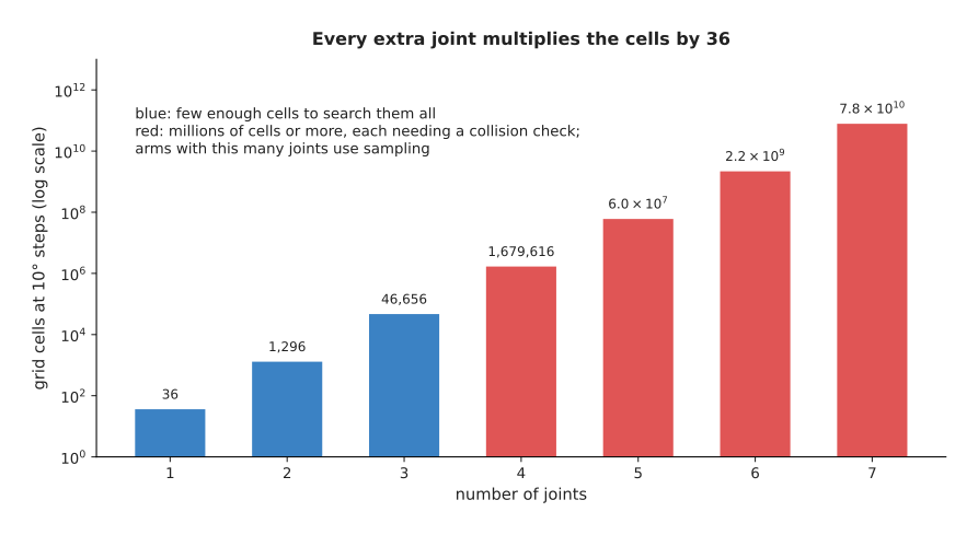
Two joints give 1,296 cells, but six joints give 2,176,782,336 cells, which is more than two billion. Each of those cells needs its own collision check before the search can use it. So a grid search, which is the subject of graph search, is a good tool only for two or three joints, or for the gripper's position alone. Instead, for a six-joint arm the usual tool is a sampling-based planner, which tests a few thousand random configurations rather than every cell.
3. The six techniques#
Because that many joints rule out a plain grid search, the chapter's pages are split into two groups. The "most used" group holds the three techniques that run on nearly every arm move. In it, a sampling-based planner finds the route, inverse kinematics turns a gripper goal into joint angles, and trajectory optimisation tidies the route. The "also used" group then holds three techniques that are common but are needed for fewer jobs. Those three are graph search for small spaces and fixed roadmaps, sampling-based optimisation and model-predictive control for fast re-planning, and visibility with next-best-view planning for moving a camera.
Here is each technique in one line, with a link to its page.
Most used
- Sampling-based planning tries random joint configurations, keeps the ones that hit nothing, and joins them up until a route appears. The rapidly-exploring random tree (RRT), RRT-Connect and the probabilistic roadmap (PRM) are the main methods, and this is what MoveIt 2 uses by default.
- Numerical inverse kinematics finds joint angles that put the gripper at a given position and direction. It starts from a guess and sees how far the gripper is from the target. It then moves the joints a little to close the gap, and repeats until the gap is small enough.
- Trajectory optimisation starts from a whole route and improves it step by step, so that the route becomes shorter and smoother and is pushed away from obstacles. CHOMP, STOMP and TrajOpt are the well-known methods that do this.
Also used
- Graph search finds the shortest or cheapest route through a network of places joined by moves, and breadth-first search, Dijkstra's algorithm and A* are the three main methods. On an arm it searches a grid of cells, or a small set of taught poses joined by known moves. The same page covers topological sort, which puts jobs in an order that respects "this before that", such as which object must be moved before another can be reached.
- Sampling-based optimisation and model-predictive control tries many random sequences of moves in a model, keeps the best, and runs only the first step before planning again. Random shooting, the cross-entropy method and CMA-ES are the main ways to choose the samples, and model-predictive control (MPC) is the plan-a-little, act-a-little loop around them.
- Visibility and next-best-view works out what a camera can and cannot see from a pose. It then chooses where to put the camera next, so that the camera sees the most of what is still unknown.
4. The six side by side#
Those one-line descriptions say what each technique does on its own. So the table below puts the six of them side by side, to show where they differ. Read each row as one technique, where the "answers" column says which part of section 1's three-part question it answers, or which other question it answers. The last column then names the most common reason that the technique fails.
| Technique | Answers | What goes in | What comes out | Same answer every run? | Usual way it fails |
|---|---|---|---|---|---|
| Sampling-based planning | which way | a collision checker, a start and a goal configuration | a route that hits nothing, usually with detours | no, it is random | a narrow gap that random samples rarely land in |
| Numerical inverse kinematics | where should the joints end up | a target pose for the gripper, a first guess | joint angles that reach it | yes, from the same guess | no answer found near a bad guess, or near a joint limit |
| Trajectory optimisation | is it good enough (and sometimes which way) | a first route, a cost, a collision distance | a shorter, smoother route with more clearance | yes, from the same first route | stuck on the wrong side of an obstacle |
| Graph search | which way | a grid or a graph, a start and a goal | the shortest or cheapest route on it | yes | too many cells when there are many joints |
| Sampling-based optimisation and MPC | which move is best right now | a model that predicts what a move does, a cost | the first step of the best sequence found, again every cycle | no, it is random | the model is wrong, or too few samples for many joints |
| Visibility and next-best-view | where should the camera go | the objects' shapes, candidate camera poses, what is still unknown | the reachable pose that would show the most | yes | objects not shaped like the model, or the best view out of reach |
Two things in the table are worth saying in words, because they change how you use the techniques.
First, the two sampling methods give a different answer each run, and Book 3's planning a path explains why that matters when a cell has to be checked and signed off.
Second, the techniques fail in different ways, so they are often used together. A sampler is good at finding some way through an awkward space, whereas an optimiser is good at making a route nice. But an optimiser can get stuck on the wrong side of an obstacle, so a common pair is a sampler that finds a route and an optimiser, or a simple shortening step, that then cleans it up.
5. How they work together on one move#
To show that pairing in action, the picture below follows one move of the book's two-joint arm. In it, link 1 is 3 m long and link 2 is 2 m long, as in Book 1. There is a box, a post and a jar on the table, and the arm must move its gripper to the star.
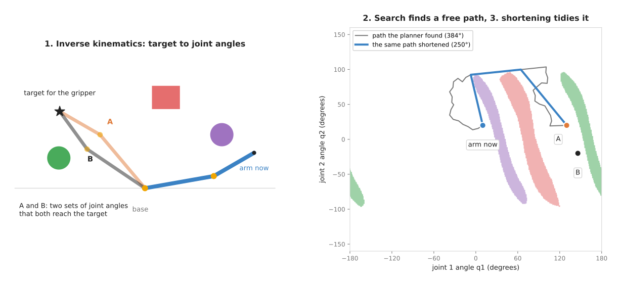
The left panel is the table seen from above, while the right panel is the configuration space. Each coloured band on the right is the set of joint angles where the arm would touch the object of the same colour on the left.
The move happens in three steps.
- Inverse kinematics turns the target into joint angles. The target is a point for the gripper, and two sets of joint angles reach it: A, at (130°, 20°), and B, at (146°, −20°). They differ in which way the elbow bends, and the program picks A.
- A planner searches for a free route. The straight line from the current joint angles to A crosses two bands, so the arm would hit the post and then the box. Instead, an RRT-Connect planner finds a route that goes over the top of both bands. On the table, that means the arm folds its elbow sharply to pass inside the post and the box. That route is 384 degrees long, counting the joint turns added together.
- A shortening step makes the route tidier. It tries to replace parts of the route with straight lines, keeping each one only if it hits nothing, and the route drops to 250 degrees, with two corners.
The numbers come from a real run of the planner, in
planning_and_search_1.py. The
shortening step used here is the simplest kind, so the
trajectory optimisation page covers
the methods that also make the route smooth and keep it clear of obstacles.
But after step 3, the route is still only a list of joint angles, because it has no times and no speeds attached to it. Trajectory generation adds those, so that the motors can follow it.
6. How this chapter connects to the others#
That one move used a camera goal, a collision checker and a motor command, which shows how planning sits in the middle of the book's seven categories. So it takes input from the first four categories and hands its result to the sixth.
- Geometry and cameras gives the planner its goal, because a camera first finds the object in pixels. Then the pinhole camera model and rigid transforms turn those pixels into a pose in the arm's frame, which inverse kinematics turns into joint angles.
- Searching and matching provides a piece that every sampling planner uses on every step, namely nearest-neighbour search, which finds the closest point already in the tree.
- Fitting and estimation and image and point cloud processing build the obstacles that the planner avoids. So a table plane fitted with RANSAC, or a cluster of points from clustering, becomes a box in the planner's list of obstacles.
- Control and motion takes the route from this chapter and makes the motors follow it.
- Decisions and task logic decides which move to plan next, and when the choice is between several places to go, it may use graph search itself.
Book 6 has learned versions of some of these techniques, because learned motion planners covers networks that suggest routes, networks that check for collisions, and networks that do inverse kinematics. That page's advice agrees with this chapter, since for moving through open space an ordinary planner is usually the better tool. This is because it is fast enough, it checks every move, and it needs no training. So learned helpers earn their place only when the same kind of problem comes up many thousands of times and the answer is needed in the same short time every run.
7. Where to read next#
Because the six pages do not have to be read in the order they are listed, the list below gives a reading order that introduces each idea before it is used.
- Start with graph search, because it explains breadth-first search, Dijkstra's algorithm and A*, which the other pages then use.
- Then read sampling-based planning, which is how most arm planners find a route.
- Trajectory optimisation and numerical inverse kinematics complete the most-used group.
- Sampling-based optimisation and MPC covers re-planning a short way ahead, many times a second.
- Visibility and next-best-view covers choosing where to point the camera.
- Book 3's planning a path covers the same planners in practice: MoveIt's defaults, the planning scene, and the ways a planner can succeed and still leave you worse off.
- Book 3's programmed methods for one arm places motion planning among the other ways to program an arm.
8. Using it in Python#
Section 5 followed one move through all six techniques, from the goal pose to the timed trajectory. What it did not say is who calls whom in real code. After this section you will know where a Python program actually joins that chain on a ROS 2 arm, which is higher up than the six techniques themselves.
The honest answer is that you do not call a planner from Python. You call
MoveIt, and MoveIt calls the planner, the inverse kinematics solver, the
collision checker and the time parameteriser in the order section 5 describes.
The Python interface to MoveIt is moveit_py, and a whole move looks like this.
import rclpy
from moveit.planning import MoveItPy
from geometry_msgs.msg import PoseStamped

rclpy.init()
robot = MoveItPy(node_name="moveit_py")
arm = robot.get_planning_component("panda_arm")

arm.set_start_state_to_current_state()

goal = PoseStamped()
goal.header.frame_id = "panda_link0"      # the frame the pose is measured in
goal.pose.position.x = 0.28
goal.pose.position.y = -0.2
goal.pose.position.z = 0.5
goal.pose.orientation.w = 1.0
arm.set_goal_state(pose_stamped_msg=goal, pose_link="panda_link8")

result = arm.plan()
if result:
    robot.execute(result.trajectory, controllers=[])
That short program reaches every technique in this chapter. set_goal_state
with a pose makes MoveIt run
numerical inverse kinematics
to turn the pose into joint angles. plan runs a
sampling-based planner from OMPL,
asking the collision checker about every sample, and then smooths the result.
The trajectory optimisation step
runs too if your planning pipeline is configured for CHOMP or STOMP. Then
execute sends the trajectory to the controller.
MoveIt does the joining, and that is a larger contribution than it sounds. It loads your arm's description, keeps the planning scene of obstacles up to date from the camera, hands the sampler a collision checker built from your arm's own shapes, converts between frames, and turns a path into a trajectory with speeds that respect your joint limits. Writing that by hand is the reason the six technique pages each end by pointing at a library rather than at a listing.
What you still have to write is everything outside the move. You write the
sequence of moves, the gripper commands between them, the recovery when plan
returns nothing, and the decision about which pose to aim for in the first
place, which is the job of Book 3's task-level chapters. You also have to write
the configuration, because MoveItPy reads a MoveIt configuration package that
names your arm's joints, its kinematics solver, its planning pipelines and its
controllers. There is no pip install that produces a working planner, because
a planner without a robot description has nothing to plan for.
What you have to decide or measure is the description of your own robot and its world. The planner needs the arm's link shapes, its joint limits, which pairs of links are allowed to touch, how much clearance you insist on, and how long it may search before giving up. Every one of those is a number about your workcell, and the six pages in this chapter are each about one part of that list. The pages that follow give the Python for the individual pieces, and they are worth reading even though MoveIt calls them for you, because when a plan fails the message you get back is about one of these pieces and not about MoveIt.