This page explains trajectory optimisation, which is a way to plan an arm's motion by starting from a rough path and improving it, step by step. The aim is a path that is short, smooth and clear of obstacles, so the page answers five questions about how that is done. What does it mean to give a path a cost? How does a program lower that cost? What do the three well-known methods, CHOMP, STOMP and TrajOpt, do differently? Where does a robot arm use this? And when does it get stuck?
It is for a reader who has met a path planner before, for example on the pages about graph search and sampling-based planning. Those planners find a route, whereas this page is about making a route good. You do not need any calculus, because the one idea borrowed from it, the gradient, is explained where it first appears.
Book 3 compares the planner families in planning a path. This page agrees with it and goes one level down, because it runs a small optimiser, so you can see every number move.
Contents#
- The idea in one sentence
- How it works · Step 1: a path is a list of waypoints · Step 2: a cost for smoothness · Step 3: a cost for being near an obstacle · Step 4: moving every waypoint downhill · Step 5: a worked example around a pot · Step 6: the same thing for a real arm · Pseudocode
- CHOMP, STOMP and TrajOpt
- Where it is used on a robot arm
- Where it works, and where it does not
- Libraries that provide it
- Why trajectory optimisation, and what it costs
- The learned alternative
- Where to read next
- Using it in Python
1. The idea in one sentence#
Write down one number that says how bad a path is, then keep nudging the path in the direction that makes that number smaller.
That number is called the cost, and a path that is long, jerky or close to an obstacle has a high cost. A path that is short, smooth and well clear of everything has a low cost instead. So the program never searches for a route from scratch, because it starts with a guess and improves it.
Here is an everyday example: think of a garden hose laid straight across a lawn, with a flower bed in the way. You do not lay a new hose. Instead you push the middle of the hose sideways, off the bed, and the rest of the hose follows, since it is all one piece. Pushing too hard at one point makes a sharp kink, so you push a little at many points. Then, when the hose is off the bed and has no kinks, you stop.
Trajectory optimisation does the same thing with numbers, so the push off the bed is the obstacle cost, and the resistance to kinks is the smoothness cost.
A word on the name is needed here. A path is the list of positions the arm passes through, while a trajectory is a path with times attached. The methods on this page treat the points as evenly spaced in time, so "smooth" also means "no sudden changes of speed". The exact timing is set afterwards, by the step on the page about trajectory generation.
2. How it works#
Section 1 gave the idea in one sentence, so the steps below take it apart, in the order a program runs them. The example is flat, with two numbers per point, so that it can be drawn. Then step 6 explains what changes for a real arm with six joints.
Step 1: a path is a list of waypoints#
The program stores the path as a list of points called waypoints, where the first waypoint is the start and the last one is the goal. Those two never move, but all the others are free to move.
The example uses 21 waypoints, with the start at (0, 0) and the goal at (10, 0). One unit is 10 cm, so the move is 1 m long. The first guess is the obvious
one, which is a straight line with the waypoints spread evenly along it, 5 cm
apart.
In the middle of the table stands a round pot, 30 cm across, and its centre is at
(5, 0.4), so it sits a little to one side of the straight line. However, the
line still goes straight through it. The program also wants a margin of 5 cm,
which means the path should stay at least that far from the pot, and not merely
miss it.
Step 2: a cost for smoothness#
Step 1 laid out the waypoints, so the next thing to write down is what makes a path smooth. The smoothness cost adds up, for every pair of neighbouring waypoints, the square of the distance between them:
smoothness = sum over i of |waypoint[i+1] - waypoint[i]|²
The squaring matters here, because two gaps of 1 cost 1 + 1 = 2, while one gap
of 0 and one of 2 cost 0 + 4 = 4. This means the cost is lowest when the
waypoints are evenly spaced and in a straight line, and a kink or a sudden jump
makes it rise fast.
For the straight first guess there are 20 gaps of 0.5 units each, so the
smoothness cost is 20 × 0.25 = 5.000. No path between these two ends can do
better, because this is the shortest, most even path there is.
Step 3: a cost for being near an obstacle#
Smoothness on its own would keep the straight line, so a second cost has to push the path off the pot. The obstacle cost looks at each waypoint's distance to the surface of the pot, and that distance is positive outside the pot and negative inside it. The cost for one waypoint is then this:
- zero when the waypoint is more than the margin away from the surface
- small and gently rising as the waypoint comes inside the margin
- large, and rising steadily, once the waypoint is inside the pot
In numbers, with d the distance to the surface and m the 5 cm margin:
if d < 0:       cost = -d + m/2               (inside the pot)
if 0 <= d < m:  cost = (d - m)² / (2m)        (inside the margin)
otherwise:      cost = 0
This is the obstacle cost that CHOMP uses, and its two pieces meet smoothly at the surface, so the cost has no sudden step. For the straight first guess, seven waypoints are inside the pot or its margin, and their costs add up to 5.316.
The program needs the distance from any point to the nearest obstacle surface, and for one round pot that is simple arithmetic. For a real scene, however, it comes from a distance field, which is a grid that stores, in every cell, the distance to the nearest occupied cell. The page on morphology and the distance transform shows how to compute one from a map of occupied cells.
Step 4: moving every waypoint downhill#
Steps 2 and 3 gave two separate costs, so the program has to add them into one number. The total cost is the smoothness cost plus the obstacle cost times a weight. That weight says how much a unit of obstacle cost counts against a unit of smoothness. The example uses a weight of 10.
total = smoothness + 10 × obstacle
Now the program has to find which way to move each waypoint so that the total goes down, and that direction is given by the gradient. The gradient of the cost at a waypoint is an arrow that points the way the cost rises fastest. So the program moves each waypoint a small distance the opposite way. This is called gradient descent, which means walking downhill on the cost, one small step at a time.
Each part of the cost gives its own arrow, and each of them has a plain meaning.
- The smoothness arrow points from the waypoint towards the middle of its two neighbours, so moving there straightens the path at that point.
- The obstacle arrow points straight away from the pot, and it is zero outside the margin.
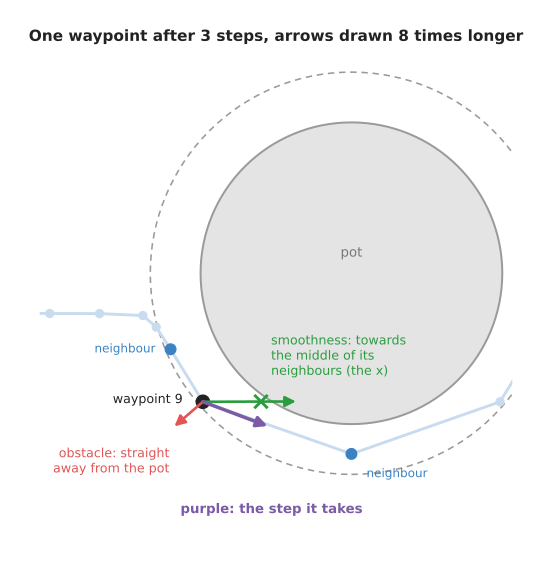
The picture shows waypoint 9 after three steps. The green arrow pulls it towards the green cross, which is halfway between its neighbours, while the red arrow pushes it away from the pot. Then the purple arrow is their sum, which is the step it actually takes.
The size of each step is the gradient times a small number called the step size, and the example uses 0.05. Too small, and the program needs thousands of steps; too large, and waypoints jump past where they should be, so the path shakes instead of settling.
Step 5: a worked example around a pot#
With the cost and the gradient both in place, the program runs 300 steps of gradient descent. The table below shows the path at a few of those steps. Read each row as one moment, with the smoothness cost, the obstacle cost, the total, the clearance, and the length of the path. The clearance is the smallest distance from the path to the pot's surface, checked all along the path and not only at the waypoints. This means a negative clearance shows that the path goes through the pot.
| Step | Smoothness | Obstacle | Total | Clearance | Length |
|---|---|---|---|---|---|
| 0 | 5.000 | 5.316 | 58.160 | -11.0 cm | 100.0 cm |
| 1 | 5.831 | 2.427 | 30.103 | -6.2 cm | 102.1 cm |
| 5 | 8.259 | 0.023 | 8.485 | 2.6 cm | 111.0 cm |
| 10 | 7.414 | 0.013 | 7.540 | 3.3 cm | 110.6 cm |
| 50 | 5.914 | 0.002 | 5.933 | 4.4 cm | 107.1 cm |
| 100 | 5.636 | 0.001 | 5.645 | 4.6 cm | 105.6 cm |
| 300 | 5.524 | 0.000 | 5.529 | 4.7 cm | 105.1 cm |
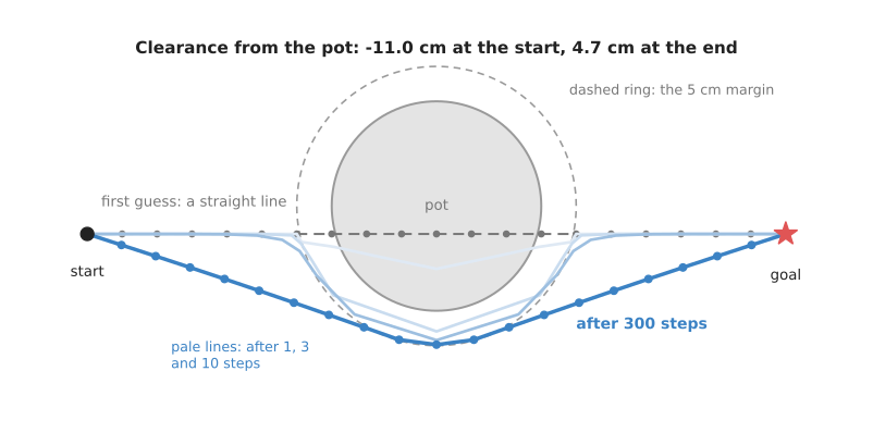
The grey dashed line is the first guess, the pale blue lines are the path after 1, 3 and 10 steps, and the dark blue line is the path after 300 steps, bending round the side of the pot that the first guess was already nearer to.
Two phases are easy to see in those numbers, and they pull in opposite directions.
In the first few steps the obstacle term wins. So the waypoints inside the pot are pushed out hard, and the path leaves the pot after three steps. It gets longer and more bent as it goes, because the smoothness cost rises from 5.000 to 8.259 by step 5. At that point the path has a sharp dent where it was pushed.
After that the smoothness term wins, because the obstacle cost is already close to zero, so the smoothness pull straightens the dent out. The path gets shorter again, from 111.0 cm at step 5 to 105.1 cm at step 300, and it spreads the bend over the whole move. After that the clearance keeps rising towards the 5 cm margin, and it ends at 4.7 cm.
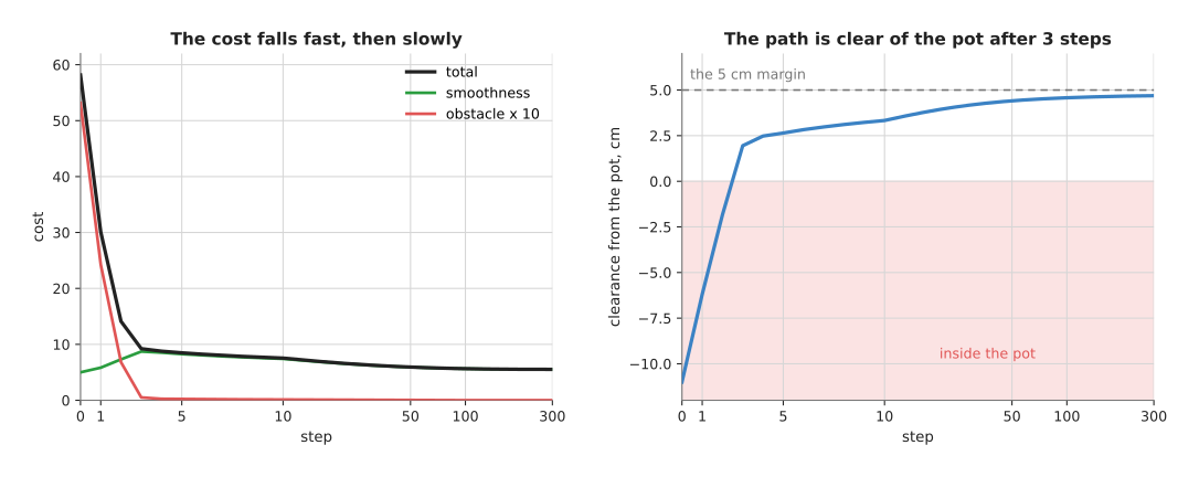
On the left, the total cost falls steeply for three steps and then slowly; on the right, the clearance crosses zero after three steps and creeps up towards the dashed 5 cm line.
The final clearance is 4.7 cm and not 5, but that is not a mistake. The margin is part of a cost and not a hard rule, so the last few millimetres cost more in smoothness than they save in obstacle cost. If you need a hard guarantee, you either add a hard constraint, which is what TrajOpt does (section 3). Instead of that, you can check the final path and set the margin a little larger than what you really need.
The whole run takes a fraction of a second in plain Python. The script that makes
the pictures, docs/diagrams/planning_and_search_2.py, runs it and prints every
number in this section.
Step 6: the same thing for a real arm#
The example so far was flat, but a real arm works in the space of joint angles, as the planning a path page explains. So three things change.
- Each waypoint is a list of joint angles, for example six numbers for a
six-joint arm, instead of an
(x, y)point. - The smoothness cost is the same sum of squared differences, now taken between neighbouring lists of joint angles.
- The obstacle cost is added up over many points on the arm's body, and not over a single point. The program places a few dozen small spheres along the links, and for each sphere it reads the distance field. Then it turns the sphere's obstacle arrow into joint-angle arrows with the arm's Jacobian. The Jacobian says how far a point on the arm moves when each joint turns a little, and the page on numerical inverse kinematics explains it with a small example.
Everything else, the weight, the step size and the loop itself, stays the same.
Pseudocode#
The pseudocode below is the loop from this section, written without any particular language.
function optimise_path(start, goal, n_waypoints, weight, step_size, n_steps):
    path = n_waypoints points evenly spaced on the straight line start -> goal

    repeat n_steps times:
        for each inner waypoint i (not the first, not the last):
            # smoothness: pull towards the middle of the two neighbours
            g_smooth = 2 * (2 * path[i] - path[i-1] - path[i+1])

            # obstacle: push away from the surface, only inside the margin
            d = signed distance from path[i] to the nearest obstacle surface
            away = unit direction from the obstacle towards path[i]
            if d < 0:           g_obstacle = -away
            else if d < margin: g_obstacle = (d - margin) / margin * away
            else:               g_obstacle = 0

            step[i] = step_size * (g_smooth + weight * g_obstacle)

        for each inner waypoint i:
            path[i] = path[i] - step[i]           # move downhill

        if the total cost has stopped falling: stop early

    check the whole path for collisions, not only the waypoints
    return path
The last line matters, because the cost only looks at waypoints, so a thin obstacle can sit between two of them. This means the final check must test the segments too.
3. CHOMP, STOMP and TrajOpt#
Section 2 ran one particular optimiser, but three methods are well known, and all three are available to ROS 2 users. Book 3 lists where each one lives in planning a path. They all share the idea of section 2. This means they differ only in how they find the downhill direction, and in how they treat the rules the path must obey.
CHOMP, covariant Hamiltonian optimisation for motion planning, is the method this page runs, and it uses the gradient of the cost, as in step 4. One extra idea gives it its name. Instead of moving each waypoint by its own arrow, CHOMP spreads each waypoint's step over its neighbours, so a push on one waypoint bends a long stretch of the path at once. In the hose example this is like pushing the hose with a flat board rather than with one finger. So the path stays smooth at every step, and fewer steps are needed.
STOMP, stochastic trajectory optimisation for motion planning, does not use the gradient at all. At each step it makes a handful of noisy copies of the current path, each with small smooth random changes. Then it works out the cost of every copy. Then it moves the path towards a weighted average of the copies, with the cheaper copies weighted much more. Because it only ever asks "what does this path cost?", STOMP works with costs that have no gradient: a cost that is simply 1 for a collision and 0 otherwise, a cost that says whether a camera can see the gripper, or a cost from a simulator.
function stomp_step(path, n_copies, noise_size):
    for k in 1 .. n_copies:
        noise[k] = smooth random change, of size noise_size, zero at both ends
        cost[k] = total_cost(path + noise[k])
    weight[k] = exp(-(cost[k] - lowest cost) / temperature), then scale to sum to 1
    return path + sum over k of weight[k] * noise[k]
TrajOpt, trajectory optimisation, treats the problem as a sequence of simpler problems. At each step it replaces the true cost with an approximation shaped like a bowl near the current path, and it solves that bowl exactly. Then it only accepts the move if the true cost really went down. Its main difference, however, is that it handles hard constraints, so rules such as "clearance at least 2 cm", "joint 3 stays within its limits" or "the cup stays level" are kept exactly, and not just encouraged by a cost. It also checks collisions between waypoints, along the swept path of the arm, which removes the thin-obstacle problem from the pseudocode above.
The table below compares the three, so read each row as one property of a method.
| CHOMP | STOMP | TrajOpt | |
|---|---|---|---|
| How it finds the next step | gradient of the cost | trying noisy copies | solving a bowl-shaped approximation |
| Needs a cost with a gradient | yes | no | yes |
| Hard rules, such as joint limits | only as extra cost | only as extra cost | kept exactly |
| Collision checked | at waypoints | at waypoints | along the swept path |
| Main cost | a distance field | many cost evaluations per step | a more complex solver |
4. Where it is used on a robot arm#
Section 3 named the three methods, so this section lists the jobs a real arm calls them for.
Smoothing a sampled path. A sampling planner such as RRT-Connect finds a route that works but zigzags, and the page on sampling-based planning shows why. That is why a common pattern is to hand that route to an optimiser as its first guess. The sampler chooses which side of each obstacle to pass, while the optimiser makes the path short and smooth. In other words, this pairs the strength of each method with the weakness of the other.
A repeated move in a fixed cell. An arm that moves parts from a conveyor to a tray makes the same move thousands of times. So an optimiser started from the same guess gives the same path every time, which a random sampler cannot promise. That matters when the cell has to be checked and signed off.
Staying well clear, not just clear. Reaching past a glass on a table, a sampler's path may pass the glass by 1 mm. So the obstacle cost with a 5 cm margin keeps the arm away from it, which leaves room for the camera's error in where the glass is.
Adding a wish to the move. When the arm carries a cup of water, the cup should stay upright. In the same way, when it scans a shelf with a wrist camera, the camera should keep pointing at the shelf. Each wish becomes one more term in the cost, or one more constraint in TrajOpt, so the same optimiser handles it.
Reusing the last answer. When the scene changes a little between cycles, for example a box moved by 2 cm, the program starts from the path it used last time. Then only a few steps are needed, because the old path is already close. That is why GPU-based planners such as cuRobo use this to replan many times a second, as planning a path describes.
Beyond collision. The same loop is used to plan a throw, to keep a welding torch at a fixed speed along a seam, or to spread effort evenly over the joints. Only the cost itself changes.
5. Where it works, and where it does not#
Section 4 listed the jobs this method does well, but it is only ever as good as its first guess. It finds the best path near that guess, and such a path is called a local minimum. This means a path from which every small nudge makes the cost higher, even though a very different path would be cheaper.
The sharpest case is a pot centred exactly on the straight line, because then every push from the pot is exactly balanced by a push from the other side. The waypoints on the left of the pot are pushed left, and those on the right are pushed right. The middle waypoint sits at the pot's centre, where "away from the pot" has no direction at all, so it is not pushed anywhere.
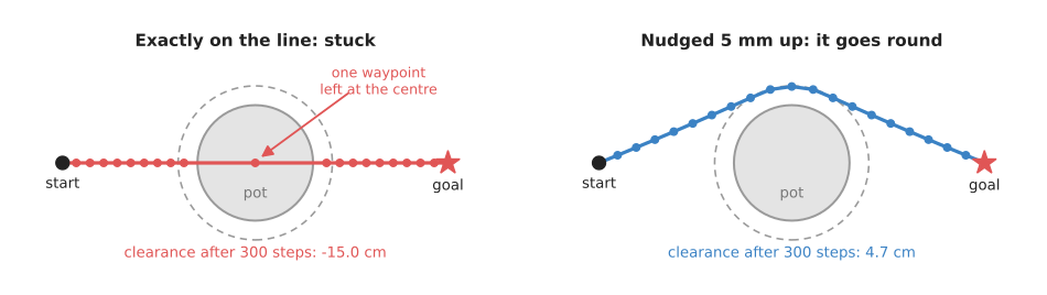
On the left, after 300 steps, the path still runs through the pot, with a clearance of -15.0 cm; on the right, the same run started with the middle waypoint moved up by only 5 mm goes round the pot and ends 4.7 cm clear.
The nudge works fast, because after one step the middle waypoint is 5.4 cm off the line. After ten steps the path is clear of the pot. Real optimisers rarely meet a case this exact, but they meet others like it all the time. For example, a path may go the long way round, or be pushed into a corner between two obstacles. The usual cures are therefore to start from a sampler's path, or to start from several guesses and keep the best.
The table below lists the common failures. Read each row as one failure, with what causes it, the sign you would see, and what people do about it.
| Failure | The sign you would see | What people do |
|---|---|---|
| Stuck in a local minimum | the cost stops falling while the obstacle cost is still above zero | start from a sampler's path, or from several guesses |
| A thin obstacle between waypoints | every waypoint is clear, yet the arm clips a shelf edge | use more waypoints, and check the segments afterwards, as TrajOpt does |
| Weight too low | the path cuts through the edge of the margin, or through the obstacle | raise the weight, or use a hard constraint |
| Weight too high | the path swings wide and has a sharp kink | lower the weight, or take more steps |
| Step size too large | the cost goes up and down instead of falling | halve the step size |
| A narrow gap | the path is pushed out of the gap and goes round, or fails | a sampler, which finds gaps by trying many points |
| A cost with no gradient | the path does not move at all | STOMP |
| The distance field is stale | the path avoids where a box used to be | recompute the field from the latest camera scan |
6. Libraries that provide it#
For a real project you use a library rather than writing this loop yourself, so the table below lists the well-known ones. Read each row as one library, with the languages you can call it from, where the method lives, and a note on when to use it.
| Library | Languages | Function, class or module | Note |
|---|---|---|---|
| MoveIt 2 | C++, Python | the CHOMP and STOMP planner plugins, in moveit_planners/chomp and moveit_planners/stomp | the usual choice in ROS 2; selected in the planning pipeline configuration |
| tesseract_planning | C++ | the TrajOpt planner, built on the trajopt packages | the maintained TrajOpt, with hard constraints and swept collision checks |
| OMPL | C++, Python | ompl::geometric::PathSimplifier, with shortcutPath and smoothBSpline | not an optimiser, but the cheap smoothing step MoveIt applies after a sampler |
| Drake | C++, Python | KinematicTrajectoryOptimization in pydrake.planning | optimises a smooth curve through joint space with constraints |
| cuRobo | Python | MotionGen | many optimisations in parallel on an NVIDIA graphics card |
| CasADi | C++, Python, MATLAB | the Opti class | write your own cost and constraints; good for special tasks |
| SciPy | Python | scipy.optimize.minimize | enough for a small experiment such as the one on this page |
For a first project, use what your planning framework already ships, which in ROS 2 is CHOMP or STOMP in MoveIt. So write your own only to learn, or when the cost is special enough that no library supports it.
7. Why trajectory optimisation, and what it costs#
With the libraries named, this section answers the four questions: what it is, what it does for you, why it rather than the obvious alternative, and what it costs.
It is a way to plan by improving a whole path at once, lowering one number that scores how long, jerky and close to obstacles the path is. It gives you a smooth path, with the clearance you asked for, and the same answer every time you ask the same question.
The obvious alternative is a sampling planner, such as RRT-Connect. A sampler is better at finding a way through a cluttered space, because it tries points all over the space instead of improving one guess. So it will find a narrow gap that an optimiser pushes the path away from. So why optimise at all? Because a sampler's path zigzags, differs every run, and passes obstacles by whatever distance it happened to find, whereas an optimiser gives the path a shape you chose, through the cost. In practice the two are used together more often than either is used alone.
Against all of that, the costs are these: you need a distance field of the scene, which takes memory and has to be recomputed when the scene changes. You also need to tune the weight and the step size, and the right values change with the task. You get no promise of finding a path when one exists. If the first guess is on the wrong side of an obstacle, the method reports a failure a sampler would have avoided. And a cost is not a rule. This means that unless you use hard constraints, as TrajOpt does, the path will trade a little clearance for a little smoothness, as the 4.7 cm in section 2 shows.
8. The learned alternative#
Section 7 weighed this method against a sampler, and Book 6 adds learned helpers for it, along with one learned way to replace it. From learned motion planners, a learned collision distance gives the obstacle cost a smooth distance without a distance field, and a learned route planner gives a quick first guess, which is what this method depends on most; the exact check still tests the final path. A diffusion or flow policy replaces the optimiser instead. It learns whole stretches of motion from people's demonstrations, so it picks one real way round an obstacle rather than a blend of them. So it wins when the right motion is easier to show than to write as a cost, such as bringing the gripper round a mug's handle. The optimiser still wins when the path must be the same every run, must keep a clearance you chose, or must avoid an obstacle nobody showed the policy. This is because a diffusion policy varies by design and does not check for collisions.
9. Where to read next#
- Numerical inverse kinematics is the next page, and it uses the same idea, a cost made smaller step by step, to find the joint angles for one pose.
- Sampling-based planning finds the first guess that this method improves, and Graph search does the same on a grid.
- The planning and search overview places this technique among the others in the chapter.
- Trajectory generation puts times on the finished path, so the motors know how fast to go.
- Morphology and the distance transform computes the distance field that the obstacle cost reads.
- Optimisation solvers covers the solvers that TrajOpt-style methods call.
- Book 3 goes deeper in planning a path, including what collision checking really checks.
10. Using it in Python#
Section 2 built the cost out of a smoothness term and an obstacle term, and section 6 said that SciPy is enough for a small experiment of exactly this kind. This section writes that experiment. After it you will be able to bend a straight guess around an obstacle in about a dozen lines, and you will understand why the version you would actually ship is a MoveIt setting rather than a Python function.
The program below is the pot example from section 2, in two dimensions. The path
is a list of waypoints, the two ends are fixed, and scipy.optimize.minimize
moves all the middle waypoints at once to make the cost smaller. SciPy works out
the downhill direction itself by trying small changes, so you do not have to
write the gradient that section 2 derives.
import numpy as np
from scipy.optimize import minimize

start, goal = np.array([0.0, 0.0]), np.array([1.0, 0.0])
centre, radius, margin = np.array([0.5, 0.0]), 0.10, 0.05   # the pot, in metres
guess = np.linspace(start, goal, 20)          # the straight line through the pot

def cost(flat):
    path = np.vstack([start, flat.reshape(-1, 2), goal])
    smooth = np.sum(np.diff(path, axis=0) ** 2)             # short, even steps
    clear = np.linalg.norm(path[1:-1] - centre, axis=1) - radius
    too_close = np.clip(margin - clear, 0.0, None)          # 0 when far enough away
    return smooth + 50.0 * np.sum(too_close ** 2)

result = minimize(cost, guess[1:-1].ravel(), method="L-BFGS-B")
path = np.vstack([start, result.x.reshape(-1, 2), goal])
Run it and the cost falls from 2.12 to 0.0575 in 117 iterations, taking a fraction of a second. The straight guess ran through the middle of the pot, with its nearest waypoint 7.4 cm inside the surface; the answer clears the pot by 4.97 cm at its waypoints, and the path is 104.5 cm long instead of 100 cm. That last number is the trade section 2 describes: the extra 4.5 cm is what the clearance cost.
SciPy does the downhill search. minimize with L-BFGS-B estimates the
gradient by finite differences, remembers the curvature it has seen, and chooses
a step length, all of which the hand-written loop in section 2 has to do by
trial and error with a fixed step size. That is why this version converges in
117 iterations where section 2's loop needed 300 steps of gradient descent.
What you still have to write is the cost, and it is worth being clear that the
cost is the entire method. The two terms above are a complete statement of what
you want: steps that are short and even, and waypoints that stay margin away
from the pot. Change the 50.0 and you change which of those two wins. Add a term
and you add a requirement, such as keeping a cup upright or keeping a joint away
from its limit. You also have to write the check at the end, because section 2's
pseudocode ends with a warning that the cost only looks at waypoints, so a thin
obstacle can sit between two of them and the final path must be tested segment
by segment.
What you have to decide or measure are the weight, the margin and the number of waypoints. The margin of 5 cm is a distance in your own workcell, and the result above shows why it is not a guarantee: the path ends at 4.97 cm and not 5, because the margin is part of a cost rather than a rule, so you set it a little larger than what you really need. The weight of 50.0 has no natural value, because it converts metres of clearance into units of smoothness, so you choose it by running the optimisation and looking at whether the path is too bent or too close. The 20 waypoints decide how finely the path can bend and how long the solve takes, and too few means a smooth curve cannot be represented at all. Finally, section 6 is right that for a real ROS 2 arm you do not write this: you select CHOMP or STOMP in MoveIt's planning pipeline configuration, which runs the same idea on the arm's real joint space with its real collision checker, and you configure the weights in a YAML file instead of in Python.