This page explains how to choose the best plan when you can score a plan but cannot take a gradient of the score. It covers three methods: random shooting, the cross-entropy method (CEM) and CMA-ES. It then covers model predictive control (MPC), which runs one of these methods again and again while the arm moves. The page answers four questions, and the first two are about the methods themselves. How does each method work, and how do they compare on the same problem? Then come the practical ones: where does a robot arm use them, and when should you use something else instead?
It is for a reader who has read the chapter overview and
trajectory optimisation. That
page improves a path by following the gradient, which is the direction in
which the cost goes down fastest. This page is about what to do instead when
there is no gradient to follow. Every number and picture on this page comes from
a real run of
planning_and_search_4.py.
Contents#
- The idea in one sentence
- The example: pushing a block past a mug
- How it works · Random shooting: try many plans, keep the best · The cross-entropy method: narrow the search · CMA-ES: also learn the shape of the search · The three on the same budget · Model predictive control: plan, do one step, look again · The pseudocode · A learned model inside MPC
- Where it is used on a robot arm
- Where it is useful, and where it is not
- Libraries that provide it
- Why sampling, and what it costs
- The learned alternative
- Where to read next
- Using it in Python
1. The idea in one sentence#
Sampling-based optimisation makes up many candidate plans, scores each one by simulating it, and uses the best-scoring ones to decide where to look next.
An everyday example shows the idea before any robot arm is involved. You are adjusting the shower, but you cannot see a formula for the water temperature, and you can only turn the tap and feel the result. So you try a few positions, notice which ones felt best, and then try a few more positions close to those. After a few rounds of this the water is right. You never worked out which way the temperature changes with the tap, because you only ever compared results. Sampling-based optimisation does the same thing, with a computer model in place of your hand under the water.
2. The example: pushing a block past a mug#
The shower needed only the tap turned, so here is a robot task with far more to choose. The example on this page is a pushing task, seen from above. A block 3 cm across starts at (0, 0) cm, and the target is (20, 4) cm. A mug stands at (10, 2) cm, right on the straight line between them. The mug is 3.5 cm in radius, so the middle of the block must stay more than 5 cm from the middle of the mug. The dashed circle in the pictures shows that limit.
The arm does not grip the block, because it only pushes it. One action is one push, in which the pusher moves by some distance to the side and some distance forwards, at most 5 cm in total. A plan is a list of 8 pushes, so one plan is made of 16 numbers in all.
To score a plan, the program needs a push model, which is a rule that says where the block ends up after a push. The model on this page is deliberately simple, and it has two parts.
- The block slides 0.8 times as far as the pusher moves, because it slips.
- It also drifts to the left by 0.15 times the push length, because the pusher meets it a little off centre.
The score of a plan is the distance from the block's final position to the target, plus 100 if the block touches the mug on the way, so a lower score is better.
This score has no useful gradient, because the "plus 100" jumps from 0 to 100 the moment the block touches the mug. A gradient tells you what a tiny change does, and here a tiny change either does nothing to that part of the score or makes it jump. The same is true of many scores on a robot, such as "did the grasp hold", "did the camera see the part", or any score that comes out of a physics simulator. Book 3's pushing and sliding explains why real pushing is hard to write as a formula at all.
3. How it works#
With the task and the score now fixed, the three methods differ only in how they choose the next batch of plans to try. They come in order below, from the simplest to the one that learns the most from each round, and then model predictive control wraps a loop around whichever one you pick.
Random shooting: try many plans, keep the best#
Random shooting is the simplest of the three, and its name comes from firing many random shots and keeping the one that lands nearest the target.
- Make up many random plans. Here each push is picked at random, up to 5 cm in any direction.
- Run each plan through the push model, and work out its score.
- Keep the plan with the lowest score.
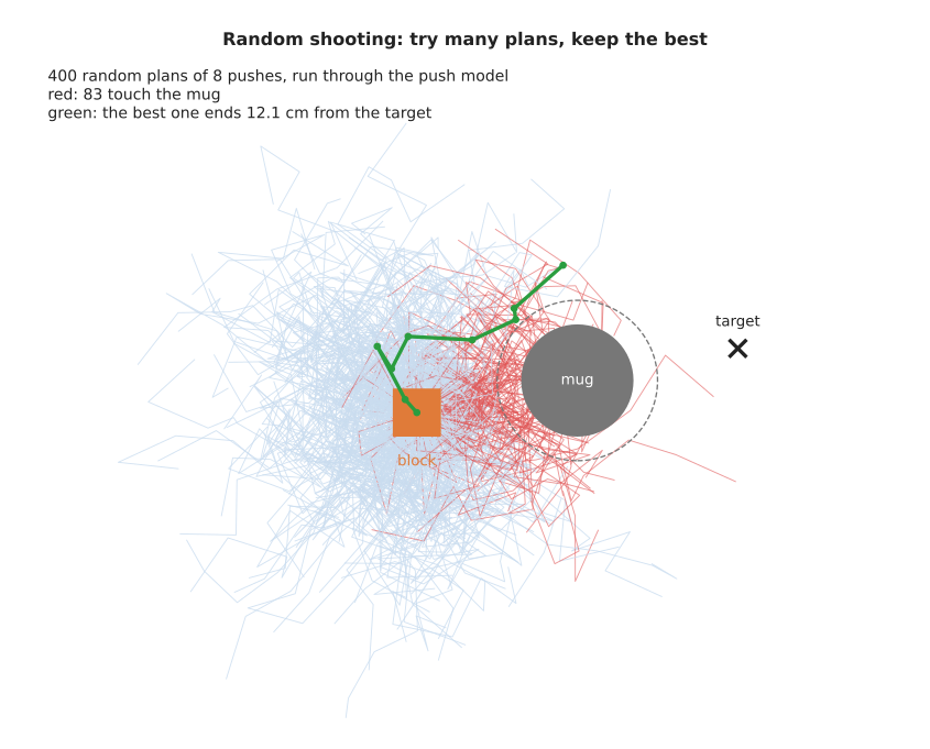
The picture shows one real run with 400 random plans. Most of them wander around the start, because random pushes cancel each other out, and 83 of them touch the mug. The best plan, in green, ends 12.1 cm from the target.
Random shooting is poor here because the plan has 16 numbers. For a good plan most of those 16 must be right at the same time, and random guessing almost never manages that. However, with only 2 or 3 numbers to choose, random shooting works well.
The cross-entropy method: narrow the search#
The cross-entropy method, or CEM, repeats random shooting, but each round it moves the search towards the best plans of the round before. The name comes from statistics, and you do not need that background to use the method.
It describes where to search with two lists of numbers. The mean is the middle of the search, with one value for each of the 16 numbers of a plan. The spread then says how far from the mean to look, again one value for each number.
- Start with a mean of zero pushes and a spread of 3 cm.
- Make 50 plans by adding random amounts to the mean, scaled by the spread.
- Score all 50, and keep the best 5. These are called the elites.
- Set the new mean to the average of the 5 elites. Set the new spread to how much the 5 elites differ from each other.
- Go back to step 2. Stop after a set number of rounds.
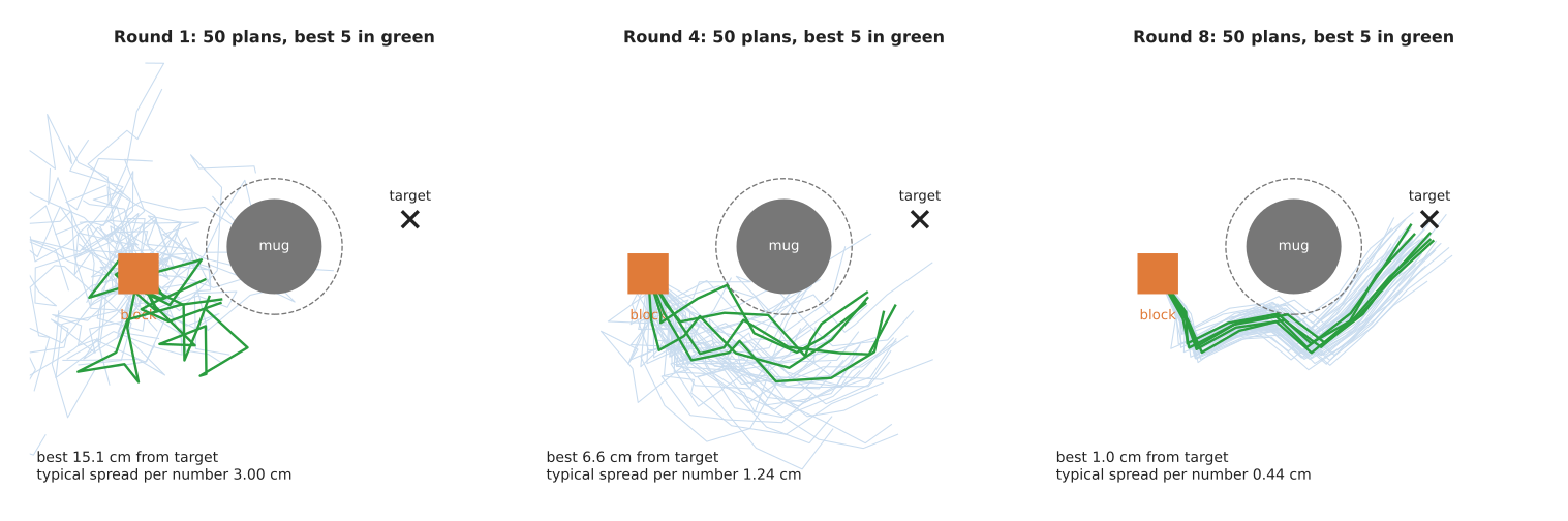
The table below gives the real numbers from that run, and you read each line as one round of 50 plans.
| Round | Best plan, cm from target | Middle plan, cm from target | Spread, cm |
|---|---|---|---|
| 1 | 15.1 | 25.9 | 3.00 |
| 2 | 10.5 | 21.2 | 2.13 |
| 3 | 8.5 | 16.0 | 1.59 |
| 4 | 6.6 | 11.9 | 1.24 |
| 5 | 4.3 | 8.4 | 0.95 |
| 6 | 2.5 | 5.8 | 0.77 |
| 7 | 1.8 | 4.4 | 0.62 |
| 8 | 1.0 | 3.0 | 0.44 |
The spread shrinks every round, and that is how CEM focuses on the good plans. It is also its weakness, because if the spread shrinks before the mean has reached a good place, the search stops moving. On this run CEM got to 1.0 cm, but on other runs it stopped further away, as the comparison below shows.
CMA-ES: also learn the shape of the search#
CMA-ES stands for covariance matrix adaptation evolution strategy, and it is the answer to that early narrowing. It keeps a mean and a spread, like CEM, but it adds two things on top.
- It learns which numbers should change together. In a push plan, pushes 3 and 4 often need to turn left together, and CEM gives each number its own spread, so it cannot say that. CMA-ES instead keeps a table, called the covariance matrix, that says how each pair of numbers should move together. The search cloud can then stretch along a slanted direction instead of only along the axes.
- It keeps a separate step size. If the last few rounds all moved the mean the same way, the step size grows, so the search moves faster. If the moves were back and forth, the step size shrinks instead. This stops the search from freezing too early, which is CEM's weakness.
The maths behind these updates is much longer than the idea, so in practice you use it from a library, as section 6 shows. The script uses the standard settings, which for a plan of 16 numbers means 12 plans per round.
The three on the same budget#
Now that all three methods have been described, the fair way to compare them is to give each one the same number of plan scores. Here each method scored 400 plans, and each ran 20 times with different random seeds. A seed is the number that starts a random number generator, so each seed gives a different run.
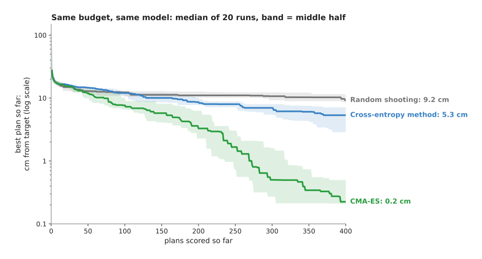
The table gives the same result as numbers, and you read each row as one method, with the distance from the target of its best plan.
| Method | Median after 100 plans | Median after 400 plans | Best run | Worst run |
|---|---|---|---|---|
| Random shooting | 12.3 cm | 9.2 cm | 7.0 cm | 12.8 cm |
| Cross-entropy method | 12.0 cm | 5.3 cm | 1.0 cm | 9.8 cm |
| CMA-ES | 7.7 cm | 0.2 cm | 0.05 cm | 3.7 cm |
On this problem CMA-ES is clearly the best, while CEM beats random shooting but often narrows too early, and this matches common practice. CEM is popular because it is ten lines of code, and because it works well on short plans with a good starting guess, which is exactly the situation inside MPC below. CMA-ES is instead the usual choice for a longer one-off search, such as tuning a set of gains.
Model predictive control: plan, do one step, look again#
All three methods above score their plans in a model, so a plan is only ever as good as that model. The real block is never exactly like the model. To show this, the script uses a "real" block that slides only 0.65 times as far as the pusher and drifts 0.30 times the push to the left. The planner does not know this, because it still uses the model's 0.8 and 0.15.
Model predictive control, or MPC, deals with this by re-planning all the time, in four steps.
- Look at where the block really is now.
- Plan a short sequence of pushes from there with the model. Here the plan is 5 pushes, found by CEM.
- Do only the first push of the plan. Throw the rest away.
- Go back to step 1.
The short plan is called the horizon, and each new plan starts from the last plan, shifted by one push, so it already starts close to a good answer. This is called a warm start, and it is why CEM is enough inside MPC.
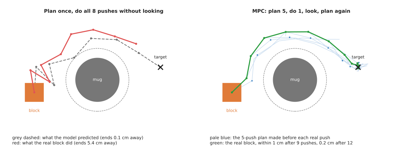
The left panel plans all 8 pushes once, with CMA-ES. In the model the plan ends 0.07 cm from the target, which is the grey dashed line. However, the real block, in red, slides less and drifts more, so it ends 5.4 cm from the target. Nothing corrected that error, because nothing ever looked at the real block.
The right panel is MPC instead, and its pale blue lines are the 5-push plans made before each real push, while the green line is the real block. Its distance to the target after each push was 17.8, 17.1, 15.6, 12.8, 9.7, 6.2, 2.9, 1.1 and then 0.3 cm, and it stayed within 0.7 cm for the last three pushes. The model was wrong every time, but each error was small and was corrected at the next look.
MPC for the block uses a slightly different score from the one-off plan. It adds up the distance to the target after every push, not only the last one, so the block gets there soon and then stays. It also adds a cost for coming within 1.5 cm of the mug's limit, and that margin is there because the model is not exact. Without it, a plan that passes the mug by a millimetre in the model can touch it in reality.
This is the same MPC that Book 3's controlling the move describes: solve a short optimisation from where you are now, do the first command, throw the rest away, and solve again. Book 3 also lists the solvers that use gradients, such as acados and Crocoddyl, while this page is the version for scores without a gradient.
The pseudocode#
The pseudocode below puts the two together, with CEM first and then the MPC loop that calls it.
function cem(state_now, mean, horizon, n_plans, n_elites, rounds):
    spread = starting spread, one value per number in a plan
    for round in 1 .. rounds:
        for k in 1 .. n_plans:
            plan[k]  = mean + spread * random normal numbers
            plan[k]  = clip each push to what the arm can do
            score[k] = score_by_simulating(state_now, plan[k], model)
        elites = the n_elites plans with the lowest scores
        mean   = average of elites
        spread = how much the elites differ from each other
    return the best plan seen

function mpc(model):
    mean = zero pushes for the whole horizon
    loop until the task is done:
        state = measure the real world now
        plan  = cem(state, mean, horizon, ...)
        do only plan's first push on the real arm
        mean  = plan without its first push, with a zero push added at the end
Random shooting is simply cem with one round and a very wide spread. CMA-ES
instead replaces the two update lines with its own updates for the mean, the
covariance matrix and the step size.
A learned model inside MPC#
The MPC above scored its plans with a push model written by hand, in which the
block slides 0.8 times as far as the pusher and drifts 0.15 times to the left.
Sometimes nobody can write such a model, and then the model can instead be
learned from records of the arm pushing the block. The planner itself does not
change at all when this happens. CEM, the horizon of 5 pushes, the warm start,
the score and "do only the first push" all stay the same. Instead, only the
prediction step inside score_by_simulating is replaced. Book 7's
learned dynamics models
page explains how such a model is built and trained.
A single learned model carries a danger that a written one does not, because the planner searches for the plan with the best predicted score. Where the model has seen no records its predictions are only guesses, and the planner is drawn to any guess that looks good. So the usual choice is an ensemble, which is several copies of the network, each trained from different random starting numbers on its own resampled copy of the records. Where the records are dense the copies agree, and where there are none they disagree. The planner therefore uses the copies' average as the prediction, and adds a cost for how far apart they end up. This keeps the plans where the model knows what happens. Only the scoring line of the pseudocode changes:
for each copy m of the ensemble:
    path[m] = roll plan[k] forward from state_now through copy m
middle   = the average of the paths
spread   = how far the paths are from middle, added up over the horizon
score[k] = score_of_path(middle) + weight * spread
The example runs in making_models_work.py,
and its "real" block differs from the one above in two ways. First, every push
has 0.15 cm of random scatter. Second, a push longer than 3 cm starts to turn the
block, so it drifts a further 0.3 cm for every centimetre beyond 3 cm. The arm
records 200 random pushes, each at most 3 cm long, and five small networks, each
with 16 hidden neurons, learn from them. Each copy's average training error is
about 0.18 cm, which is about the size of the scatter.
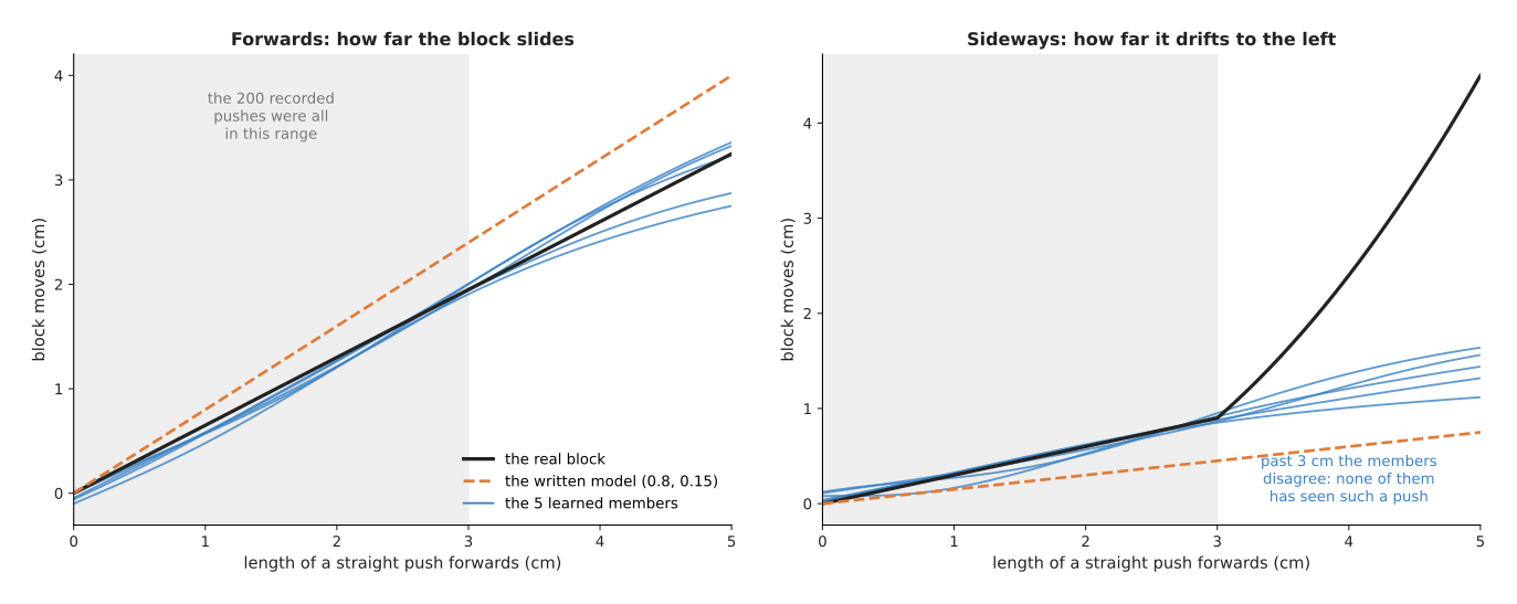
Up to 3 cm the five copies sit on the real block's line, and they are closer to it than the written model is. At 3 cm they end 0.05 cm apart on average. Beyond 3 cm, where there are no records, they spread to 0.17 cm apart at 4 cm, and to 0.30 cm apart at 5 cm. None of them knows about the extra drift, so that spread is the only warning the planner ever gets.
Each version of MPC then ran 60 times on the real block, with 12 pushes per run. You read each row of the table below as one prediction step inside the same planner.
| Prediction step | Median distance from target at the end | Runs ending within 1 cm | Runs that touched the mug | Pushes longer than 3 cm |
|---|---|---|---|---|
| Written push model | 0.6 cm | 51 of 60 | 22 of 60 | 72% |
| Learned ensemble, average only | 0.6 cm | 50 of 60 | 26 of 60 | 58% |
| Learned ensemble, plus a cost of 0.5 per cm of spread | 0.5 cm | 55 of 60 | 13 of 60 | 53% |
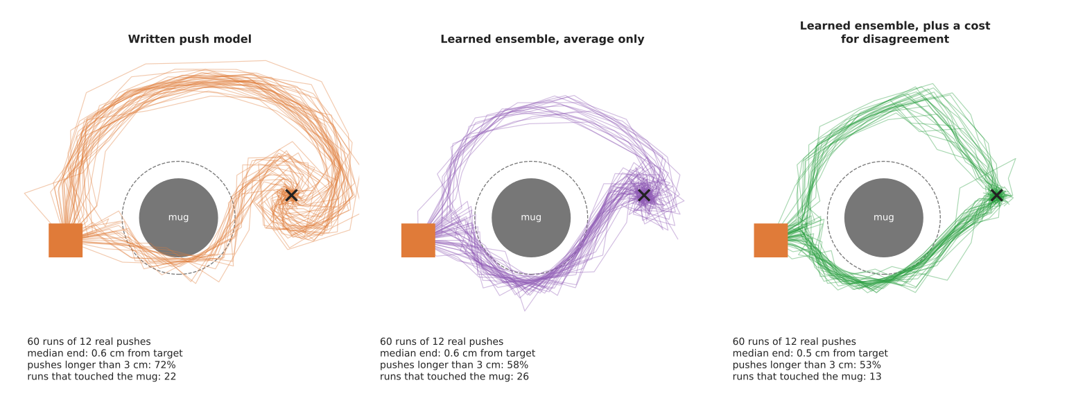
The learned model on its own was no better than the written one. It was accurate where it had records, but the planner still chose long pushes, where it was only guessing. With the cost for disagreement the planner chose fewer long pushes, and the runs that touched the mug fell from 26 to 13 of 60. However, sixty runs is only just enough to show this, because the 95% confidence intervals are 30.6% to 56.8% and 12.1% to 34.2%, which barely overlap. Book 7's evaluation and failure page explains these intervals.
The weight on the spread is itself a setting to choose, and too much of it makes the planner timid. With a weight of 2 instead of 0.5, only 4 of 60 runs touched the mug, but only 4 of 60 ended within 1 cm, and the median run ended 3.9 cm short. In other words, the planner refused the long pushes it needed. PETS, described on the Book 6 page, is the standard published version of this method, and mbrl-lib in section 6 provides it.
4. Where it is used on a robot arm#
The pushing example is one case of a wider pattern, because sampling-based optimisation is used wherever a program can simulate a plan but cannot differentiate the result. Here are the concrete places it turns up on an arm.
- Pushing and sliding objects. An arm may push a mug out of the way before a grasp, or slide a box against a wall. The contact is hard to model with a clean formula, so a sampled plan through a rough model, corrected by MPC, is common.
- MPC with a learned model. Book 7's learned dynamics models plan with CEM and MPC through a neural network. The network has a gradient, but it is often unreliable, and CEM only needs the network's predictions. PETS, listed on that page, is the standard example.
- Tuning controller gains. The gains of a PID controller can be scored by running a test move and measuring the overshoot and the settling time, so CMA-ES can tune a handful of gains this way, in simulation or on the real arm.
- Choosing a grasp. Book 7's grasp quality models use CEM to refine grasp candidates towards the ones the model scores highest.
- Paths with costs that have no gradient. STOMP, on the trajectory optimisation page, is sampling-based optimisation applied to a whole path. MPPI, model predictive path integral control, is the same weighted-average idea used inside MPC.
- Fitting a model to measurements. When a simulator has unknown settings, such as friction, CMA-ES can choose the settings that make the simulator match recorded data, which is one approach to system identification.
5. Where it is useful, and where it is not#
All of those uses rely on the same small requirement, because these methods need only one thing, which is a way to score a plan. That makes them easy to apply, but it also means they know nothing about the problem beyond the scores they see.
The table below lists the common problems, and you read each row as a problem, the sign you would see, and what people do instead.
| Problem | The sign you would see | What people do instead |
|---|---|---|
| Too many numbers in a plan | scores stop improving; plans look random | a shorter horizon, fewer numbers per push, or a gradient method |
| CEM narrows too early | every run stops at a different, mediocre plan | more plans per round, a minimum spread, or CMA-ES |
| Scoring is slow | each plan takes seconds, so a search takes hours | run many plans at once on a graphics card, or a cheaper model |
| The model is wrong | the plan looks perfect in simulation and fails on the arm | MPC, which re-plans from the real state; a margin around obstacles |
| MPC too slow for the control rate | the arm waits between pushes, or jerks | fewer plans, warm starts, or MPC only for the slow outer loop |
| A score with a smooth, known gradient | sampling takes far more evaluations than needed | trajectory optimisation or a solver |
| A hard safety limit | sometimes a plan breaks the limit | a separate safety check, as Book 3 says MPC cannot replace a safety stop |
The last row is the one that matters most, because a sampled plan satisfies a rule only as far as its score punishes breaking it, and only in the model. So anything that must never happen needs its own check outside the optimiser.
6. Libraries that provide it#
Because the methods themselves are small, CEM is short enough that most people write it themselves, as the pseudocode shows. CMA-ES is longer, so a library is the safer choice there. The table below lists well-known ones, and you read each row as one library, the languages it serves, the names to look for, and a note.
| Library | Languages | Function or class | Note |
|---|---|---|---|
| pycma | Python | cma.CMAEvolutionStrategy, cma.fmin | the reference CMA-ES, by its author |
| Optuna | Python | optuna.samplers.CmaEsSampler | CMA-ES inside a tuning framework; handy for gains |
| Nevergrad | Python | the CMA optimiser and many others | a collection of gradient-free optimisers |
| MuJoCo MPC | C++ | the Predictive Sampling planner, among others | MPC in the MuJoCo simulator; Book 3 recommends it for building intuition |
| pytorch_mppi | Python | MPPI | sampling MPC on a graphics card, with any model you give it |
| mbrl-lib | Python | CEMOptimizer | CEM and MPC for learned dynamics models, in the PETS style |
For a first try, write CEM in NumPy around your own model and score. Then move to pycma when the plan has more than a handful of numbers and CEM stops improving.
7. Why sampling, and what it costs#
With the methods, the uses and the libraries covered, this section answers the four questions for sampling-based optimisation: what it is, what it does for you, why it rather than the obvious alternative, and what it costs.
It is a family of methods that choose a plan by scoring many candidate plans in a model and moving the search towards the best ones. MPC then wraps it in a loop that re-plans from the real state after every step. Together they let an arm act well with only a rough model and a score, even when the score jumps, as it does when a block touches a mug.
The obvious alternative is a gradient method, such as the trajectory optimiser of this chapter. When a smooth gradient exists, a gradient method needs far fewer evaluations, and it scales to hundreds of numbers. However, it cannot use a score that jumps, a simulator it cannot look inside, or a learned model whose gradient is unreliable, while sampling can use all three. So choose sampling when the score has no useful gradient and the plan has tens of numbers rather than thousands. Choose a gradient method instead when the cost is smooth and you can write it down.
The second alternative is to plan once and then carry the plan out blind. That is cheaper, but the left panel of the MPC picture shows what happens, because a plan that was perfect in the model missed by 5.4 cm on the real block. MPC costs a new search at every step, and in return it corrects that error for free.
The costs come in five parts, and the first is the sheer number of evaluations, because one decision takes hundreds or thousands of model runs. The second is that the result is random, so two runs give different plans. The third is that there is no guarantee of the best plan, only of a good one. The fourth is a dependence on the model, which MPC reduces but does not remove. The fifth is the settings you must choose, which are the number of plans, the number of elites, the horizon and the spread. On this page's problem, the choice of method alone changed the result from 9.2 cm to 0.2 cm.
8. The learned alternative#
A learned model inside MPC in section 3 keeps the search and learns only the prediction, but the other learned alternative replaces the search itself. A policy that learns without a model, such as a reinforcement learning policy, turns the state straight into the next action in one pass, with no rollouts at each step. So it wins when each decision must be fast and the task stays fixed. However, Book 6 says it needs far more attempts to learn, and it learns only one task, while MPC with a model can push the block to a different mark tomorrow just by changing the score. So choose MPC when the goal changes, or when the search fits in the time between steps.
9. Where to read next#
- Trajectory optimisation covers the gradient methods, and STOMP, the sampling method for whole paths.
- Book 3's controlling the move covers MPC in practice, and the gradient-based MPC libraries.
- Book 7's learned dynamics models explains the learned model that CEM and MPC most often plan through.
- Book 3's pushing and sliding explains the physics behind the pushing example on this page.
- Optimisation solvers covers the exact solvers for problems that can be written as equations.
- PID control explains the gains that CMA-ES is often used to tune.
10. Using it in Python#
Section 3 gave the cross-entropy method and the model predictive control loop as pseudocode, and section 6 advised writing the cross-entropy method yourself in NumPy before reaching for a library. This section does both, on the pushing task from section 2. After it you will have the shortest honest version of each, and you will see exactly where the line between your code and a library falls on this page.
The first block is the cross-entropy method, written out. It is short on purpose, because section 6 is right that this is a method most people write rather than install. The second block replaces it with pycma, which is CMA-ES written by the person who invented it.
import numpy as np
import cma

target, mug, keep_out = np.array([20.0, 4.0]), np.array([10.0, 2.0]), 5.0

def score(plan):
    """Simulate 8 pushes and return how far the block ends from the target."""
    block, hit = np.zeros(2), False
    for push in plan.reshape(-1, 2):
        length = np.linalg.norm(push)
        if length > 5.0:                      # the arm cannot push further than 5 cm
            push, length = push / length * 5.0, 5.0
        left = np.array([-push[1], push[0]]) / length
        block = block + 0.8 * push + 0.15 * length * left   # slip, and drift left
        if np.linalg.norm(block - mug) < keep_out:
            hit = True
    return float(np.linalg.norm(block - target) + (100.0 if hit else 0.0))

# The cross-entropy method: 8 rounds of 50 plans, keeping the best 5 each time.
rng = np.random.default_rng(0)
mean, spread = np.zeros(16), np.full(16, 3.0)
for _ in range(8):
    plans = mean + spread * rng.standard_normal((50, 16))
    costs = np.array([score(p) for p in plans])
    elites = plans[np.argsort(costs)[:5]]
    mean, spread = elites.mean(axis=0), elites.std(axis=0)
# The same search, with CMA-ES from pycma instead of the loop above.
best_plan, best_score, found_at = cma.fmin(score, np.zeros(16), 3.0,
                                           {'maxfevals': 400, 'seed': 1})[:3]
Running the first block prints a best plan 15.1 cm from the target after round 1 and 2.2 cm after round 8, with the spread shrinking from 3.00 cm to 0.43 cm, which is the narrowing that section 3 describes. Running the second block on the same score with a budget of 400 simulations reaches 0.23 cm. That gap is the argument of section 3 for CMA-ES: on the same budget it learns the shape of the search as well as its position, so it keeps improving after the cross-entropy method's spread has collapsed.
pycma does the sampling, the update of the mean, the update of the covariance
matrix and the step size control, which together are several hundred lines that
are easy to get wrong. cma.fmin returns a long tuple, and the first three
entries are the best plan, its score, and the evaluation number at which that
plan was found.
What you still have to write is score, and on this page that is not a detail
but the entire content. A sampling optimiser knows nothing except how to ask
"what does this plan cost", so the model of how the block slides, the keep-out
distance from the mug and the penalty for touching it are all yours. That is
also why the method is worth knowing: score contains an if that jumps by
100, and section 2 explains that such a jump has no useful gradient, so no
gradient-based optimiser can use this function at all. For model predictive
control you also write the outer loop from section 3, which measures the world,
plans, does only the first push, shifts the mean along by one step and plans
again.
What you have to decide or measure is the model inside score, the budget, and
the starting spread. The 0.8 slip and the 0.15 drift are measurements of your
own pusher on your own surface, so you get them by pushing a real block and
recording where it ends up, and section 3 warns that a wrong model gives a
confident plan that fails on the robot. The budget is 50 plans times 8 rounds
here, and on a real arm it is set by how long you can afford between control
cycles rather than by what converges best. The starting spread of 3 cm has to
cover the useful plans without wasting the first rounds on absurd ones, and
section 3 shows that if it collapses before the mean has reached a good place,
the search simply stops. Finally, the 100 for touching the mug is a choice: it
has to be large enough that no plan buys distance by clipping the mug, which you
check by looking at whether the best plan ever touches it.