This page explains how a program splits a mask or a point cloud into separate objects. It answers four questions, and the first two are about grouping things that lie close together: how a program numbers the separate blobs in a mask, and how it groups 3D points into objects by how close they are. The other two ask how DBSCAN does the same while also marking stray points as noise, and why a point cloud is usually thinned out onto a grid of small cubes before any of this runs. A later section then adds two methods that look for the centre of each crowd of points instead. Those two are k-means, which must be told how many groups there are, and mean shift, which is not.
It is for a reader who already knows what a mask and a point cloud are. A mask is a picture in which each pixel is either "object" or "not object", and the page on thresholding and colour masks makes one. A point cloud is a list of 3D points, one for each depth pixel, that a depth camera measures on the surfaces in front of it.
Clustering is the step that turns "these pixels, or these points, are not table" into "this is object 1, this is object 2 and this is object 3". Almost every programmed perception pipeline on a robot arm needs it, because the arm picks one object at a time.
Contents#
- The idea in one sentence
- How it works · Connected components: blobs in a mask · Euclidean clustering: groups of nearby points · DBSCAN: nearby points, with a noise rule · Voxel downsampling: preparing the cloud · Choosing the distance
- Finding the peaks: k-means and mean shift · K-means: k centres, moved to the average · Mean shift: every point climbs to its crowd · Where each fits on a robot arm · Where they fail · Libraries
- Where it is used on a robot arm
- Where it works, and where it does not
- Libraries that provide it
- Why clustering, and what it costs
- The learned alternative
- Where to read next
- Using it in Python
1. The idea in one sentence#
The whole technique fits into one sentence, and the rest of this page fills that sentence in. Clustering puts two pixels or two points in the same group whenever they are close enough to each other, and it keeps doing so until every group stops growing.
For an everyday example, scatter some rice, some lentils and a few coins on a dark table and look at it from above. You see three heaps and a few loose grains, and you do not need to know what rice is in order to see those heaps. You see them because the grains in one heap touch each other, while there is bare table between one heap and the next. Clustering uses the same rule, so it does not know what the objects are, and it only knows which points are near which.
This is why clustering works on objects the robot has never seen before. It is also why it fails when two objects touch, because then there is no bare table between them.
2. How it works#
That one rule takes three different forms, so this section covers three grouping methods and one preparation step. Connected components works on a mask, which is a grid of pixels, whereas Euclidean clustering and DBSCAN work on a point cloud, where the points have no grid. Voxel downsampling then thins a point cloud before it is clustered.
A point cloud of a table scene normally goes through two steps before clustering. First, points that are too far away are cut off. Second, the table itself is found and removed, usually with RANSAC. What is left is a set of points that are not table, and those are the points that clustering splits into objects.
Connected components: blobs in a mask#
Connected components gives every separate blob in a mask its own number. Two object pixels belong to the same blob if you can walk from one to the other by stepping only on object pixels.
So the only choice left is what counts as a step. With four-connectivity you may step up, down, left or right, while with eight-connectivity you may also step diagonally. The difference matters when two blobs touch only at a corner.
The method itself is a flood fill, which is the same thing as the paint-bucket tool in a drawing program.
function connected_components(mask, neighbours):   # neighbours: 4 or 8 steps
    label = a grid of zeros, the same size as mask
    next_label = 0
    for each pixel p in mask, row by row:
        if mask[p] is object and label[p] is 0:
            next_label = next_label + 1
            label[p] = next_label
            queue = [p]
            while queue is not empty:
                q = take one from queue
                for each step s in neighbours:
                    n = q + s
                    if n is inside the grid and mask[n] is object and label[n] is 0:
                        label[n] = next_label
                        add n to queue
    return label, next_label
Here is a worked example, in which the picture below shows a mask 10 pixels wide and 7 high, labelled both ways.
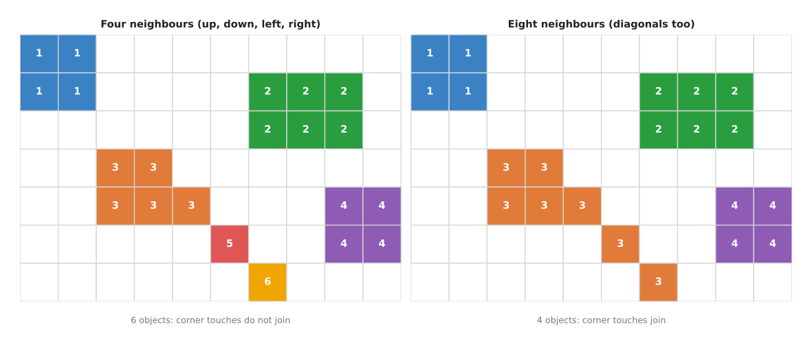
Each coloured square is an object pixel, and the number on it is the label the flood fill gave it.
With four-connectivity the program finds 6 blobs, because blob 3, blob 5 and blob 6 form a diagonal line of pixels. They touch only at corners, so four-connectivity keeps them apart. With eight-connectivity the diagonal steps are allowed, so these three join into one blob and the program finds 4 instead. Neither answer is wrong, so the choice depends on the job. You choose eight-connectivity when a thin diagonal part, such as a wire, should stay in one piece, and four-connectivity when objects that touch only at a corner should stay apart. OpenCV and scikit-image use eight-connectivity by default, while SciPy uses four-connectivity, so check which one your library uses.
Once each blob has a number, the program can measure each one, giving its area in pixels, its bounding box and its centroid. It then throws away blobs that are too small to be an object, so this size filter removes the specks of noise left over from the threshold.
The flood fill visits each pixel a fixed number of times, so its time grows in step with the number of pixels. This means that on a camera picture it takes about a millisecond.
Euclidean clustering: groups of nearby points#
A point cloud has no grid, so "neighbour" cannot mean "the next pixel" any more. Instead, two points are neighbours if the straight-line distance between them is below a chosen value, and that value is called the cluster tolerance. The word "Euclidean" just means this ordinary straight-line distance.
Euclidean cluster extraction is then the same flood fill as above, with that new meaning of "neighbour".
function euclidean_clusters(points, tolerance, min_size):
    label = -1 for every point            # -1 means "not yet in a group"
    groups = []
    for each point p:
        if label[p] is not -1: skip it
        start a new group g containing p; label[p] = g
        queue = [p]
        while queue is not empty:
            q = take one from queue
            for each point n within tolerance of q:    # a radius search
                if label[n] is -1:
                    label[n] = g
                    add n to queue
        add g to groups
    throw away every group with fewer than min_size points
    return groups
The line "each point within tolerance of q" is a radius search. Written
simply, it compares q with every other point, which is slow for a large cloud.
So real libraries build a k-d tree first, and then each search only looks at
nearby points. The page on
nearest-neighbour search
explains how.
Here is a worked example, in which the points below are what is left on a table after the table plane was removed, seen from above. There is a round cup, a box, a small block and 7 scattered stray points, which is 323 points in all. The points on each object are about 6 mm apart, with a little random noise, and the objects are at least 43 mm apart.
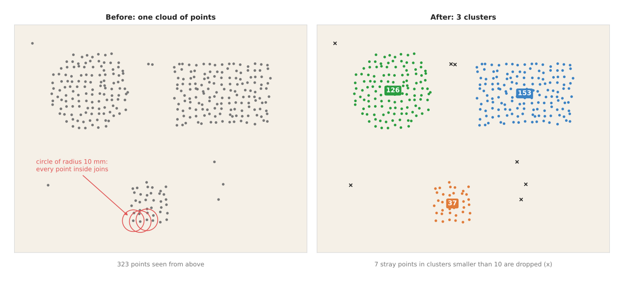
The left panel shows the points before clustering, with the 10 mm circle round three points of the block. The right panel shows the result, with the size of each cluster written on it.
With a tolerance of 10 mm, the flood fill first finds 9 groups: the box with 153 points, the cup with 126, the block with 37, one pair of stray points and five single stray points. A minimum size of 10 points then throws away the 6 small groups, so the result is 3 clusters, which is right. These numbers come from running the code behind the picture on these points.
DBSCAN: nearby points, with a noise rule#
Euclidean clustering has one known weakness, which is that it chains. If A is near B and B is near C, then A, B and C are one group, even if A and C are far apart, so a thin line of stray points between two objects joins them into one cluster. Such lines are common, because depth cameras make stray points along the edges of objects, and a cable or a speck of dust can lie between two parts.
DBSCAN, short for "density-based spatial clustering of applications with
noise", fixes this with one extra rule. It sorts every point into one of three
kinds, using a radius eps (the same idea as the tolerance) and a count
min_pts.
- A core point has at least
min_ptspoints, counting itself, withineps. It sits in a crowded area, such as the middle of an object's surface. - A border point is not a core point, but it lies within
epsof a core point. It sits on the edge of a crowded area. - A noise point is neither. It sits alone.
Clusters then grow as Euclidean clusters do, with one change: a cluster only keeps growing from core points. So a border point joins the cluster, but the search does not continue from it, and noise points join nothing at all.
function dbscan(points, eps, min_pts):
    for each point p:
        near[p] = all points within eps of p           # includes p itself
        core[p] = (size of near[p] >= min_pts)
    label = -1 for every point                         # -1 means noise
    next = 0
    for each point p:
        if not core[p] or label[p] is not -1: skip it
        label[p] = next
        queue = [p]
        while queue is not empty:
            q = take one from queue
            for each n in near[q]:
                if label[n] is -1:
                    label[n] = next
                    if core[n]: add n to queue         # only core points spread
        next = next + 1
    return label
The picture below runs DBSCAN on the same 323 table points, with eps of 10 mm
and min_pts of 5.
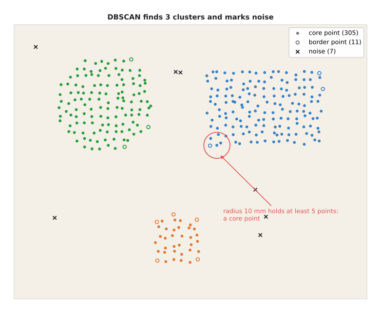
Filled dots are core points, open circles are border points, and crosses are noise; the red circle shows the 10 mm radius round one core point.
DBSCAN finds the same 3 clusters, of 153, 126 and 37 points. Of the 323 points, 305 are core points, 11 are border points and 7 are noise. The border points sit on the corners and outer edges of the objects, because a point there has fewer neighbours. The 7 noise points are exactly the stray points that Euclidean clustering removed with its size filter, so here the two methods agree.
However, they disagree when stray points form a bridge, and the picture below shows two blocks 30 mm apart with a line of 4 stray points between them.
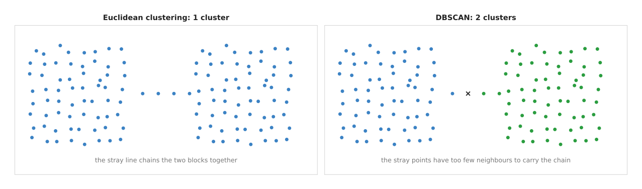
The same 132 points and the same 10 mm distance give one cluster on the left and two on the right.
The stray points are about 7 mm apart, so each one is within 10 mm of the next.
Euclidean clustering therefore walks along the line from one block to the other,
and it reports one cluster of 132 points. DBSCAN counts neighbours first, and
three of the four stray points have only 3 points within 10 mm, counting
themselves, which is below min_pts of 5. So they are not core points, and the
search cannot pass through them. This means DBSCAN reports two clusters of 65 and
66 points, and marks 1 point as noise.
DBSCAN's min_pts looks as though it does two jobs at once, and Book 2 warns
about mixing them. It is a noise filter, which decides whether a point sits in a
crowded area, so it is not a size filter for whole objects. This means a program
still throws away clusters that are too small, as a separate step. Book 2's
choosing the grouping distance
works through both numbers for a real camera.
Voxel downsampling: preparing the cloud#
A depth camera with 640 by 480 pixels gives up to 307,200 points per picture, and clustering them all is slow. It is also not needed, because two points 1 mm apart on the same surface tell the program nothing new. So the cloud is thinned out first.
Voxel downsampling divides space into small cubes of equal size, and each cube is called a voxel, short for "volume pixel". Every cube that holds at least one point is then replaced by a single point, which is the average of the points inside it.
function voxel_downsample(points, size):
    for each point p:
        cell = (floor(p.x / size), floor(p.y / size), floor(p.z / size))
        add p to the list for that cell
    return, for each cell with points, the average of its points
The picture below does this in 2D, seen from above, for a dense scan of a mug and a box.
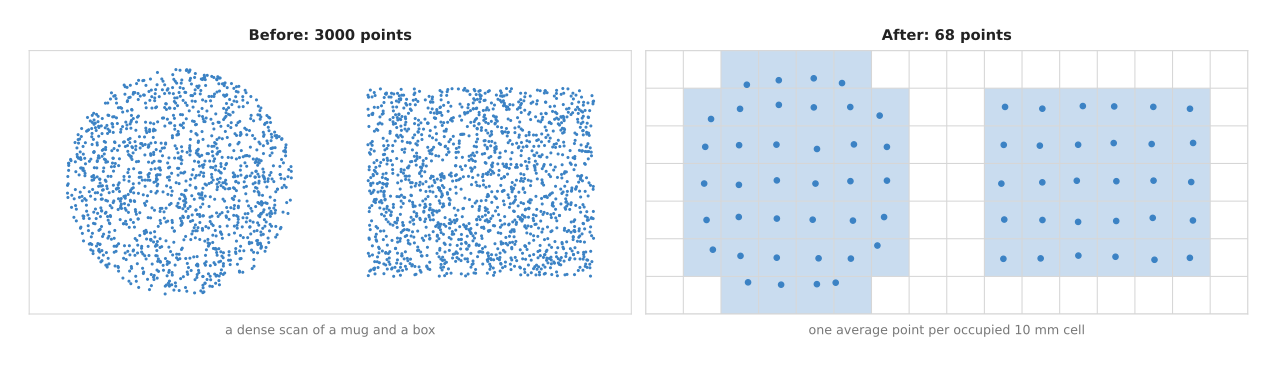
The left panel has 3,000 points, while the right panel has one average point for each occupied 10 mm cell, which comes to 68 points.
The table below shows how the cell size sets the number of points left from the same 3,000. Read each row as "with cubes of this size, this many points remain".
| cell size | points left | share of the original |
|---|---|---|
| 5 mm | 245 | 8.2% |
| 10 mm | 68 | 2.3% |
| 20 mm | 26 | 0.9% |
Downsampling does three useful things for clustering. It makes clustering much faster, because there are far fewer points to search through. It also makes the point spacing even, so one tolerance works everywhere: near the camera the points are crowded and far away they are sparse, and the grid removes that difference. It then averages away some of the depth noise as well.
It also sets a limit on the tolerance. After downsampling, the points on one surface are about one cell apart, and up to one cell diagonal apart. A cube of side 10 mm has a diagonal of 10 × √3 = 17.3 mm. So the cluster tolerance must be larger than that, or one object will break into several clusters. The page singulation and pre-grasp manipulation works through this link between the cell size and the tolerance, using the settings from the Point Cloud Library's own tutorial.
Choosing the distance#
Every method so far rests on one number, because the tolerance, or eps, is the
setting that decides the result. It must lie between two limits.
- It must be larger than the gaps between points on one object. If it is smaller, one object breaks into many small clusters.
- It must be smaller than the gap between two objects. If it is larger, two objects join into one cluster.
The table below shows this on the 323 table points, with Euclidean clustering and a minimum size of 10. Read each row as "with this tolerance, the program keeps these clusters and drops this many points".
| tolerance | clusters kept (points in each) | points dropped |
|---|---|---|
| 5 mm | none | 323 |
| 6 mm | 11 pieces, from 47 down to 10 points | 114 |
| 8 mm | 3 (153, 126, 37) | 7 |
| 20 mm | 3 (153, 126, 37) | 7 |
| 30 mm | 2 (281, 37) | 5 |
| 50 mm | 1 (322) | 1 |
At 5 mm and 6 mm the tolerance is below the point spacing, so the objects shatter. From 8 mm to 20 mm the answer is right and does not change, whereas at 30 mm the cup and the box join, together with two stray points, and at 50 mm everything joins. So the wide range from 8 mm to 20 mm with the same answer is what you look for when you tune, and you pick a value in the middle of it. The robot-arm-projects repository explains the same two limits for glasses on a table, in plain words, in cluster on the table.
One more trick helps a great deal, because objects on a table all stand on the same plane. If the program first flattens the points onto that table plane and clusters in 2D, then the height of the objects no longer matters. So a tall object and a short one next to it are compared only by the gap between them on the table.
3. Finding the peaks: k-means and mean shift#
Every grouping method in section 2 uses one rule, which is that two points are in the same group if a chain of close neighbours joins them. This section covers two methods with a different rule, because they look for centres, meaning places where points crowd together. Each point then belongs to the centre it is nearest to, or to the centre it climbs to.
The two methods differ in one important way. K-means must be told how many groups to find, whereas mean shift finds the number for itself. Section 7 says that k-means is the wrong tool for counting objects, because on a robot the number of objects is usually the thing you want to find out. That is still true. However, there are jobs on a robot arm where the number of groups is known in advance, and there k-means is the simplest tool. There are also jobs where you want the crowded middle of each group rather than the whole group, and mean shift is made for those.
For an everyday example, imagine a school with three buses, where each child must walk to one bus stop. K-means is the planner who is told "place three stops", and the planner puts the stops where they make the total walking shortest. Mean shift is what happens with no planner at all. Each child walks towards where most other children are standing, again and again, until the children stand in a few tight crowds. So the number of crowds is whatever it turns out to be.
K-means: k centres, moved to the average#
K-means has one setting, which is k, the number of groups, and it works in
rounds.
- Choose
kstarting centres. The simplest way is to pickkof the points at random. - Put every point in the group of its nearest centre.
- Move each centre to the average of the points in its group.
- Repeat steps 2 and 3 until the centres stop moving.
function kmeans(points, k):
    centres = k points picked at random
    repeat:
        for each point p:
            group[p] = the index of the centre nearest to p
        new_centres = for each group, the average of its points
        if new_centres == centres: stop
        centres = new_centres
    return group, centres
Here is a worked example on a job where k is known in advance. A camera looks
at red and blue parts on a grey table, and the program must find the three colours
in the picture, so that it can build a colour mask for each kind of part. Each
pixel's colour has a red amount and a blue amount, each from 0 to 255. So each
pixel can be drawn as one point, with its red amount across and its blue amount
up. The picture has 500 pixels: 300 of table, 120 of red parts and 80 of blue
parts.
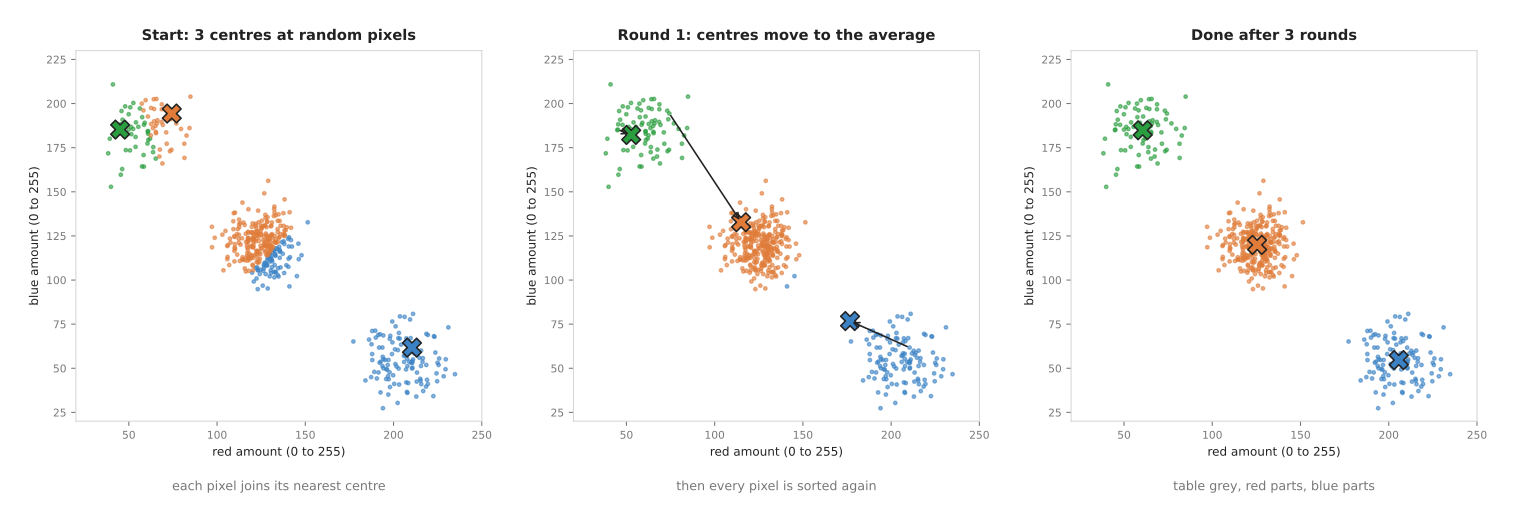
In each panel, the crosses are the centres and each dot is coloured by the centre it is nearest to.
The random start here is poor, because it picks one red pixel and two blue pixels, and no table pixel at all. After the first round, the orange centre has moved from (74.3, 194.4) to (115.0, 132.8), because most of its group was table pixels. The blue centre has moved from (210.4, 61.7) to (176.7, 76.8), pulled towards the table. After 3 rounds the centres are at (205.7, 54.6), (60.6, 184.9) and (125.4, 119.9), and a fourth round changes nothing, so the method stops. The groups then hold exactly 120, 80 and 300 pixels, which is one group per real colour.
A start can be so poor that k-means stops at a wrong answer. Out of 10 different random starts on these pixels, 8 give the answer above, while the other 2 end with two centres inside one colour and one centre between the other two colours. The fix is simple, because you can run k-means several times from different starts and keep the answer with the smallest spread, which is the sum, over all pixels, of the squared distance to their centre. Libraries do this for you, and they also choose the starts more carefully, with a method called k-means++ that picks starting centres far apart from each other.
The picture below shows what happens when k itself is wrong, and each panel
keeps the best of 10 starts.
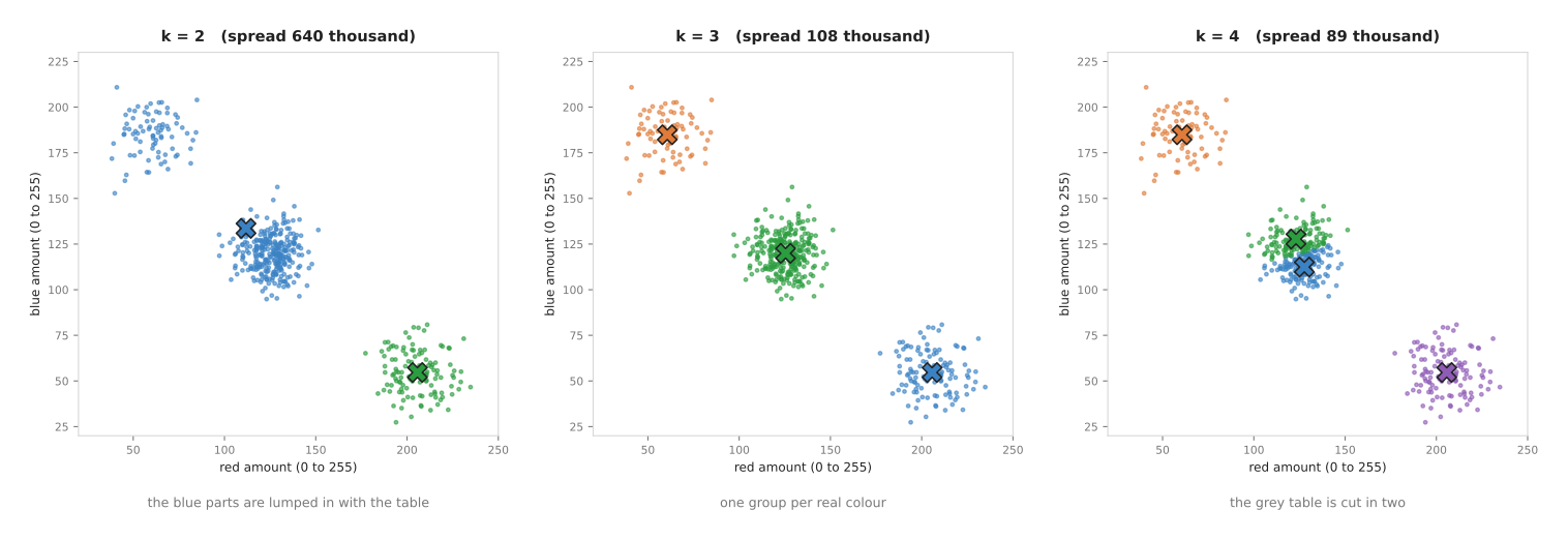
With k = 2, the blue parts are lumped in with the table, and the spread is
640,122. With k = 3, the spread drops to 108,302. With k = 4, the grey table
is cut into two halves of 153 and 147 pixels, and the spread drops again, to
89,061. So a smaller spread does not mean a better answer, because the spread
always falls as k grows, until every pixel is its own group. The usual sign of
the right k is where the spread stops falling steeply. So here the fall from
640,122 to 108,302 counts as a big drop, while the fall from 108,302 to 89,061 is
a small one.
Mean shift: every point climbs to its crowd#
Mean shift has one setting too, but it is a distance rather than a count, and it is called the bandwidth or the window. The method treats the points like a hilly landscape, where the ground is highest where the points are most crowded. So from each point it climbs uphill until it reaches a top, which is called a peak.
- Put a round window of the chosen radius on a starting point.
- Move the window's centre to the average of all points inside the window.
- Repeat step 2 until the window stops moving. Where it stops is a peak.
- Do this from every point. Peaks that end up very close together are one peak.
- Each point belongs to the peak it climbed to.
The average of the points in the window always lies a little further into the crowd than the window's centre, because more points sit on the crowded side. This means every step moves uphill.
function mean_shift(points, window):
    peaks = []
    for each point p:
        c = p
        repeat:
            near = all points within window of c
            new_c = the average of near
            if distance(new_c, c) is tiny: stop
            c = new_c
        if c is within window / 2 of a peak already in peaks:
            label[p] = that peak
        else:
            add c to peaks; label[p] = the new peak
    return peaks, label
Here is a worked example, in which a grasp model looked at a table with a mug, a box and a small block. It proposed 150 grasp centres, seen from above and measured in millimetres: 70 round the mug, 45 round the box, 20 round the block and 15 scattered at random. The arm wants one grasp per object, at the middle of each crowd of proposals.
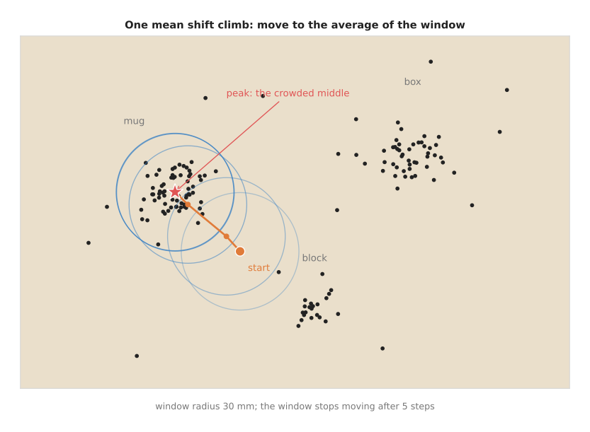
The picture follows one climb, with a window of radius 30 mm, and it starts at (112, 60), between the mug and the block. The average of the points in the first window is (105.0, 67.6), which is a small step towards the mug. The next window holds more mug points, so the next step is bigger, to (85.4, 83.9). Then comes (79.0, 90.1), and then (78.8, 90.3), where the window stops moving. The mug's proposals were spread round the point (80, 90), so the peak is within 2 mm of it.
Run from all 150 points with the same 30 mm window, mean shift finds 7 peaks, and the 3 largest are reached from 72, 49 and 23 points. They lie at (78.8, 90.3) for the mug, (198.5, 108.3) for the box and (149.1, 32.0) for the block. The other 4 peaks are reached from only 1 or 2 points each. This is because they are stray proposals with no crowd round them, so a size limit throws them away, just as in section 2.
The window is the one number that matters here, and the picture below runs the same points with three different windows.
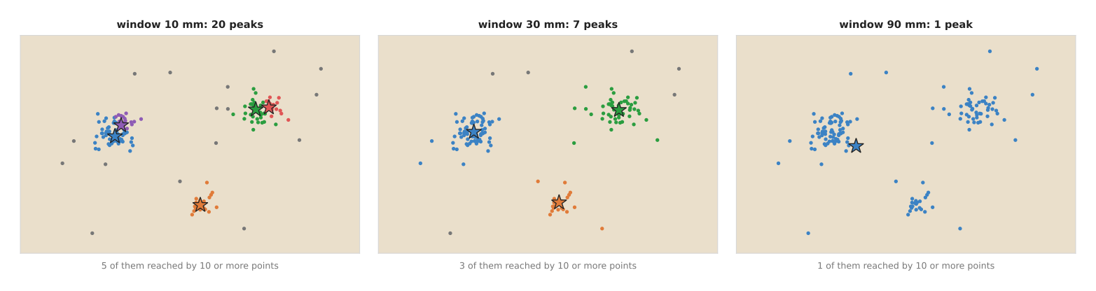
Coloured dots belong to peaks reached from 10 or more points, and grey dots belong to the small peaks.
The table below gives the full result for six windows. Read each row as "with this window, mean shift finds this many peaks, and this many of them are reached from at least 10 points".
| window | peaks found | peaks reached from 10 or more points |
|---|---|---|
| 10 mm | 20 | 5 (the mug and the box each split in two) |
| 20 mm | 12 | 3 |
| 30 mm | 7 | 3 |
| 45 mm | 4 | 3 |
| 60 mm | 3 | 3 |
| 90 mm | 1 | 1 (at (98.8, 78.5), between the objects) |
A window from 20 mm to 60 mm gives the three right crowds, and that wide, steady range is what you look for, as with the tolerance in section 2. A window that is too small splits one crowd into several, whereas a window that is too large joins everything into one peak, which may lie on bare table between the objects.
Where each fits on a robot arm#
K-means therefore fits the jobs where the number of groups is fixed in advance by the job itself.
- Finding the colours of a known set of parts. As in the example, k-means
finds the
kmain colours in a picture. Their centres give the colour ranges for the masks on the thresholding page, and they adapt when the light changes. - Choosing
kspread-out options. A planner may want 5 different approach directions, or 4 camera viewpoints, out of hundreds of candidates. K-means on the candidates giveskgroups, and the program takes the best candidate from each. - Splitting a pile you have already counted. If a weighing scale or a
barcode says the tray holds exactly 3 parts, k-means with
k= 3 splits the tray's points into 3 groups, even where connected components sees one blob.
Mean shift, by contrast, fits the jobs where you want the crowded middle and the count is unknown.
- Merging many proposals into a few. A grasp model, an object detector run on several frames, or several camera views each give many nearby guesses for the same object. Mean shift turns each crowd of guesses into one answer at its middle, as in the example.
- Finding vote peaks. Some pose models let every pixel of an object vote for where the object's centre is. Mean shift finds the peak of those votes. It is the same job as finding the peak in the Hough transform's vote table, without a table of cells.
- Following a coloured object in a video. OpenCV's
meanShiftandCamShiftclimb a picture that holds, for each pixel, how well its colour matches the object. Started at the object's last position, the window climbs to its new position in each frame.
Where they fail#
K-means fails in four ways. With the wrong k, objects merge or split, as in the
picture above. From a poor start it can also stop at a wrong answer, and you would
see a different answer on each run, so use k-means++ starts and several runs. It
expects groups that are round and of similar size. So a long thin object such as a
pen gets split, and a big group steals points from a small one next to it.
Finally, a few far-away points pull a centre away from its crowd, because every
point counts in the average. So for objects on a table, the methods of section 2
are usually the better choice.
Mean shift fails in three ways. With a poor window, peaks split or merge, as the table above shows. It is also slow on large clouds, because each step of each climb searches all the points, so it is run on a few hundred proposals rather than on 300,000 camera points. So downsample first, or start climbs only from a grid of seed points. Finally, a peak can lie between two objects when the window is large, as in the 90 mm panel. So always check a peak against the points near it before sending the arm there.
Libraries#
OpenCV provides cv::kmeans, with cv::KMEANS_PP_CENTERS for k-means++ starts
and an attempts setting for several runs, and cv::meanShift and
cv::CamShift for following an object in a video. scikit-learn provides
sklearn.cluster.KMeans, which uses k-means++ and several runs by default,
sklearn.cluster.MiniBatchKMeans for very many points, and
sklearn.cluster.MeanShift, with sklearn.cluster.estimate_bandwidth to suggest
a window from the data. SciPy provides scipy.cluster.vq.kmeans2.
4. Where it is used on a robot arm#
Both families of method serve the same need, because clustering is used wherever a program has "not background" and needs "separate objects". The list below gives concrete places.
- The table-top pick pipeline. Take the depth picture as a point cloud, downsample it, remove the table plane with RANSAC, cluster the rest, and pick the cluster nearest the gripper. This is the most common programmed perception recipe for arms. Book 2 describes it in point clouds: remove the plane, then cluster, and the tools and libraries page shows it as real Open3D code.
- Counting objects. The number of clusters is the number of objects. A tray check can compare it with the number of parts that should be there.
- Splitting a colour mask into objects. After an HSV threshold finds "red pixels", connected components splits them into one blob per red block, and the program measures each blob's centre.
- Checking whether objects touch. If two objects the robot knows are there come back as one cluster, they are closer than the tolerance. The arm can then push them apart before it grasps, as the singulation page describes.
- Removing noise before other steps. DBSCAN's noise points, or clusters below the minimum size, are thrown away before fitting shapes or computing grasps. This stops a stray point from moving an object's centre.
- Building a map of obstacles. A motion planner often keeps the scene as a grid of occupied voxels. Voxel downsampling is the same operation, and the voxels it produces can be passed straight to the collision checker used by the sampling-based planners. The page on volumetric maps explains how such a map is built from many depth pictures.
- Grouping detections over time. When several camera views each see an object, their 3D centres form small groups in space. Clustering those centres gives one position per object, ready for assignment and matching.
5. Where it works, and where it does not#
All of those uses share the same conditions, because clustering works best when objects stand apart on a known surface, the depth measurements are good, and the objects are about the same size. So it fails in a few common ways.
The table below lists them. Read each row as: this is what goes wrong, this is what you would see, and this is what people use instead.
| what goes wrong | the sign you would see | what people use instead |
|---|---|---|
| Objects touch or stand closer than the tolerance | One cluster is twice the expected size, or has a strange shape | Push them apart first; the distance transform and watershed on the morphology page; a learned segmentation model |
| The tolerance is smaller than the point spacing | One object comes back as many small clusters | Raise the tolerance above the voxel diagonal, or use a finer voxel size |
| Stray points bridge two objects | Two objects join under Euclidean clustering | DBSCAN with a min_pts that stray points cannot reach; a statistical outlier filter before clustering |
| Point density varies a lot, for example near and far objects | Far objects break up, or near objects join | Voxel downsampling first; HDBSCAN, a version of DBSCAN that adapts to density |
| The table plane was not fully removed | Every object joins the table's leftover edge into one large cluster | Remove points a few millimetres above the plane as well; crop to the work area |
| Glass or shiny objects | The object has few or no depth points, so it is missing or broken into pieces | Look for the hole in the depth picture instead, as Book 2 describes in the depth hole; a colour picture with a trained model |
| One object has two parts with a gap, such as a mug and its handle | The handle becomes its own small cluster | Merge clusters whose bounding boxes overlap; use a larger tolerance if objects stand far apart |
6. Libraries that provide it#
Because those failures are well known, so are the methods themselves, and every method on this page is available in well-known libraries. Read the table below as: this library, used from these languages, provides this method under this name.
| library | languages | function or class | note |
|---|---|---|---|
| OpenCV | C++, Python, Java | cv::connectedComponents, cv::connectedComponentsWithStats | Labels a mask. The second version also returns each blob's area, bounding box and centroid. |
| SciPy | Python | scipy.ndimage.label | Connected components on a NumPy array of any number of dimensions, so it also works on a voxel grid. |
| scikit-image | Python | skimage.measure.label, skimage.measure.regionprops | Labelling, then measuring each blob. |
| Open3D | Python, C++ | PointCloud.cluster_dbscan (C++: ClusterDBSCAN) | DBSCAN on a point cloud. Returns a label for each point, with -1 for noise. |
| Open3D | Python, C++ | PointCloud.voxel_down_sample (C++: VoxelDownSample) | Voxel downsampling with one average point per voxel. |
| PCL | C++ | pcl::EuclideanClusterExtraction | Euclidean clustering with a tolerance, a minimum size and a maximum size. Uses a k-d tree for the radius search. |
| PCL | C++ | pcl::VoxelGrid | Voxel downsampling. |
| PCL | C++ | pcl::ConditionalEuclideanClustering, pcl::RegionGrowing | Clustering with an extra rule, such as similar colour or similar surface direction, so touching objects can sometimes be split. |
| scikit-learn | Python | sklearn.cluster.DBSCAN, sklearn.cluster.HDBSCAN | DBSCAN and its density-adapting version, on any array of points. |
| scikit-learn | Python | sklearn.cluster.KMeans, sklearn.cluster.MeanShift | K-means and mean shift from section 3. |
| OpenCV | C++, Python, Java | cv::kmeans, cv::meanShift, cv::CamShift | K-means, and mean shift for following an object in a video. |
7. Why clustering, and what it costs#
With the libraries in hand, the remaining question is when to reach for clustering at all. So this section answers the four standard questions: what it is, what it does for you, why it rather than the obvious alternative, and what it costs.
Clustering is a set of flood-fill rules that group pixels or points by how close they are. Connected components does it on a grid of pixels, while Euclidean clustering does it on 3D points with a distance. DBSCAN then adds a rule that keeps stray points out, and voxel downsampling prepares the points so that the other steps run fast.
What it does for you is split "not background" into separate objects without knowing what those objects are. So it works on a part the robot has never seen, on the first day, with no training data at all. It has one main setting, the distance, and that setting can be worked out from the camera's point spacing and the smallest gap between objects.
There are two obvious alternatives. The first is k-means, which is the clustering method most people meet first, and it must be told how many groups to find. On a robot, the number of objects is usually the thing you want to find out, so k-means is the wrong tool for that job. However, Euclidean clustering and DBSCAN find the number for themselves. K-means is still useful when the number of groups is fixed by the job, such as the colours of a known set of parts, and section 3 shows where. The second alternative is a trained segmentation model or point cloud model, and section 8 says when each is the better choice.
Against all that, clustering merges objects that touch, and nothing in the method itself can fix that. You must choose the tolerance, the minimum size and the voxel size, and they depend on each other and on the camera's distance from the table. It also needs good depth, so glass and shiny metal are hard. And a radius search on a large cloud is slow unless you downsample first and use a k-d tree.
8. The learned alternative#
That second alternative is worth a closer look, because two kinds of model in Book 6 do this job. A segmentation model gives one mask per object in the colour picture, and the depth points inside each mask become that object's points. A point cloud model names every 3D point directly. Either one can split objects that touch, which clustering cannot do, and it can also say what each object is. However, a model needs labelled training data and a computer that can run it, and it only knows the kinds of object it was trained on. So choose clustering when objects stand apart, or when the robot can push them apart, and choose a model when touching objects are the normal case. Book 7's Gaussian mixture models are the learned cousin of k-means: each cluster becomes a soft, stretched blob, and every point gets a chance of belonging to each cluster instead of one hard answer.
9. Where to read next#
- The previous page is edges and contours. It traces the outline of each blob that connected components finds.
- Morphology and the distance transform tidies a mask before labelling it, and can split two touching blobs that clustering would merge.
- Nearest-neighbour search explains the k-d tree and the radius search that make clustering fast.
- RANSAC removes the table plane before clustering.
- The chapter overview compares all the techniques in this chapter.
- Book 2's methods you write yourself goes deeper into choosing the grouping distance for a real camera, and singulation and pre-grasp manipulation covers what the arm does when objects touch.
- The diagrams in section 2 are drawn by
docs/diagrams/image_processing_2.py. Every number in that section comes from the functions in that script; run it with--numbersto print them. The k-means and mean shift pictures in section 3 are drawn bydocs/diagrams/image_processing_3.py, which also takes--numbers.
10. Using it in Python#
Section 2 explained Euclidean clustering and DBSCAN, and it ended on the distance you have to choose. Section 6 named the calls. This section is the call, on a point cloud, with the choice of distance shown rather than described. After it you will be able to split a cloud into separate objects, and you will be able to see for yourself what happens when the distance is wrong.
The program below takes a cloud that has already had its table removed by the
RANSAC page's
segment_plane, thins it out, and groups the rest. It uses Open3D, which is the
point cloud library for Python, and it needs only two calls.
import numpy as np
import open3d as o3d

cloud = o3d.io.read_point_cloud("objects.ply")     # the table already removed

# Thin the cloud out: one average point per 5 mm cube.
small = cloud.voxel_down_sample(voxel_size=0.005)

# Group points that are within 20 mm of each other, in groups of 10 or more.
labels = np.array(small.cluster_dbscan(eps=0.02, min_points=10))

for k in range(labels.max() + 1):                  # -1 means noise, so skip it
    group = np.asarray(small.points)[labels == k]
    print(len(group), group.mean(axis=0))          # size and centre of one object
On a made-up cloud of two 60 mm boxes standing 90 mm apart, the downsampling
turns 3000 points into 2344, and cluster_dbscan with a 20 mm distance finds
two groups of 1141 and 1203 points, whose centres are 150 mm apart, with no
point left as noise. Change that one number to eps=0.10 and the same call returns one group
instead of two, because 100 mm is larger than the 90 mm gap and the two boxes
become one object. Nothing in the output warns you: it is a successful call with
a wrong answer.
Open3D does the neighbour search and the grouping. voxel_down_sample replaces
all the points in each small cube with their average, which both speeds up what
follows and evens out the density, and section 2 explains why uneven density
breaks the grouping. cluster_dbscan returns one label per point in the same
order as the points, using −1 for a point that belongs to no group, so the
labels line up with small.points and you index one with the other.
What you still have to write is everything that turns a group of points into an
object. The call gives you numbers of points, and you work out from them what
you need: the centre, the size, the bounding box, and whether a group is
plausibly one object at all. You also have to decide what to do with the noise
points, because a handful of scattered points may be sensor noise or may be a
thin object that failed min_points. And you have to write the step before the
call, because clustering a cloud that still contains the table produces one
enormous group, which is why the table removal comes first.
What you have to decide or measure is eps, and this page is mostly about that
one number. It has to be larger than the spacing between points on a single
object, which after voxel_down_sample(voxel_size=0.005) is about 5 mm, and
smaller than the smallest gap between two objects you need to keep apart. Those
two facts give you a range, and the 20 mm above sits in it for boxes on a table
at a typical arm working distance. So you measure the point spacing from your
own cloud rather than copying a number, and you check the result by counting the
groups against what you know is on the table. min_points is the second
decision, and it trades noise against small objects: raising it silently drops
the smallest real object, and section 2 explains that a distant object has fewer
points than a near one even when both are the same size.