This page judges this solution. It says where the solution is strong and where it breaks. It names the general ideas behind it, and places it beside the other solutions. Then it asks whether more demonstrations would help.
Contents#
- Where it is strong and where it breaks
- The general ideas behind this
- Where it sits among the others
- More demonstrations, and a result that did not come back
1. Where it is strong and where it breaks#
The earlier pages showed how the solution works. This section adds up its strengths and weaknesses.
It has four strengths. First, it is trained on the kind of input it will be shown, so the domain gap is closed. Solution 5 cannot claim this. Second, its demonstrations cost nothing, because the teacher is a program. Third, its training fits on a laptop, and it costs the same to run as solution 5. Fourth, it is one half of the cleanest comparison in the book.
It also needs no reward function. A reward is a score, but this problem has rules. Written as a penalty, "never topple a glass" becomes a price, and a policy may choose to pay a price. Copying correct pushes keeps "never topple" as a rule. The teacher kept it, and the shared check keeps it again.
Its weaknesses come in four groups. How it works explains each one where it arises.
- Some come from the borrowed model. It has about 450 million parameters, and many of them serve a language part this task does not use. It commits to a whole chunk. It cannot explain what it did. And its correction is low-rank, so it may not get all that fine-tuning could give.
- Some come from its teacher. It cannot push better than solution 2. Its training set held only successes. It saw no refusals, so it proposes pushes on glasses that must not be pushed.
- Some come from training on one examiner. It gets better here and worse elsewhere. Part of its gain is this examiner's friction stored as a fixed value. And it is random, so one run is not a measurement.
- Some jobs it does not do at all. It does not refuse, choose destinations, own the loop, or stop a push that goes wrong. The shared machinery does all of these.
These strengths and weaknesses come from standard ideas. The next section names them.
2. The general ideas behind this#
The strengths and weaknesses above come from a few standard ideas. None was invented for glasses. Each is worth knowing on its own, including when it is the wrong tool.
Transfer learning and fine-tuning#
Take a model trained on a large general task, keep its weights, and continue training on new data. This works because early layers learn general things, such as edges in pictures or smoothness in motion. Yosinski and colleagues (arXiv:1411.1792) measured this for vision. They showed that a layer transfers less well the deeper it is.
It is usually right when data for the real task is scarce. It is usually wrong when data is free and the new task looks nothing like the old one. Then the borrowed weights bring knowledge you do not need, and fix the model's size too. This solution is between those two cases. Its data is free, and its inputs are unlike the borrowed data. Solution 3 takes the other side of this choice. For more, see transfer learning.
Low-rank adaptation#
Add a small correction through a narrow squeeze, instead of changing every weight. The method is LoRA, from Hu and colleagues (arXiv:2106.09685). It is the standard way to adapt a large model on modest hardware.
It is right when the model is too large to train fully and the new task is close to the old one. It is weak when the new task is far away. It buys nothing when the model is small enough to train fully for the same money. Here the model is small and the task is far. So the result is a lower bound, as how it works explains.
Behaviour cloning, and its ceiling#
Record what an expert did, and train a model to copy it. There is no reward and no trial and error. The expert is the ceiling, and DAgger is the standard repair for the states the expert never visits. Solution 3 explains both.
Domain adaptation#
A model trained on one kind of data and used on another works across a domain gap. The methods for closing it are called domain adaptation. Fine-tuning on data from the new domain is the simplest of them. It is also the strongest, when such data exists.
When such data cannot be had, harder methods are needed. One is domain randomisation. It varies the training data so widely that the new domain falls inside it. This is the usual way to move a simulator policy to a real robot. It would be needed before this policy reached a real table, because this policy has learned one examiner's friction as a fixed value.
Catastrophic forgetting#
A network trained on a new task tends to lose what it knew of the old one. McCloskey and Cohen first described this for simple networks. Kirkpatrick and colleagues (arXiv:1612.00796) protect the weights that mattered most to the old task.
It matters when a model must stay good at several things. It matters little here, because the model is only wanted for one examiner. Low-rank adaptation also softens it, because the borrowed weights are never overwritten.
Overfitting and the held-out split#
A model can learn chance details of its examples instead of the skill. The standard defence is to train on one part of the data and test on another. The usual difficulty is that data is scarce. Here it is not, because tables are generated from numbers. For more, see overfitting.
Action chunking#
Predict a short run of actions in one pass, instead of one action at a time. ACT does this, and so does SmolVLA. Solution 3 explains why it suits pushing and what it costs.
These ideas explain the method. The next section shows where its score puts it among the six solutions measured so far.
3. Where it sits among the others#
The ideas above explain how the solution behaves. This section places its measured score beside the others.
The solutions form a ladder, ordered by how much of each one was fitted in this cell. This solution is at the top, because all of its fitting is done on a borrowed model.
Against solution 5, only the training differs. Solution 5's comparison explains why this is the cleanest pair. Two limits apply. The correction is low-rank, so the gap is a lower bound. And the reading of the waypoints must be fair to both, or the gap measures that too.
The measurement gives an answer this book did not expect. The training worked as training. The trained model's chunks are much closer to the teacher's, and it brings the jaw down to the table. But it made the score worse. The numbers below come from the first fit, on the first band of 800 tables, with one seed. Each is the median of three runs over the 50 held-out tables. Where the demonstrations come from describes both bands.
- About three pushes in five are blocked on the way down: 227 of 369. The jaw comes down onto a glass, because the model never learned where to put it down.
- 40 glasses fall over in a run. Solution 5 topples 12.
- 36 of the 50 tables are marked wrong. Solution 5 has 9.
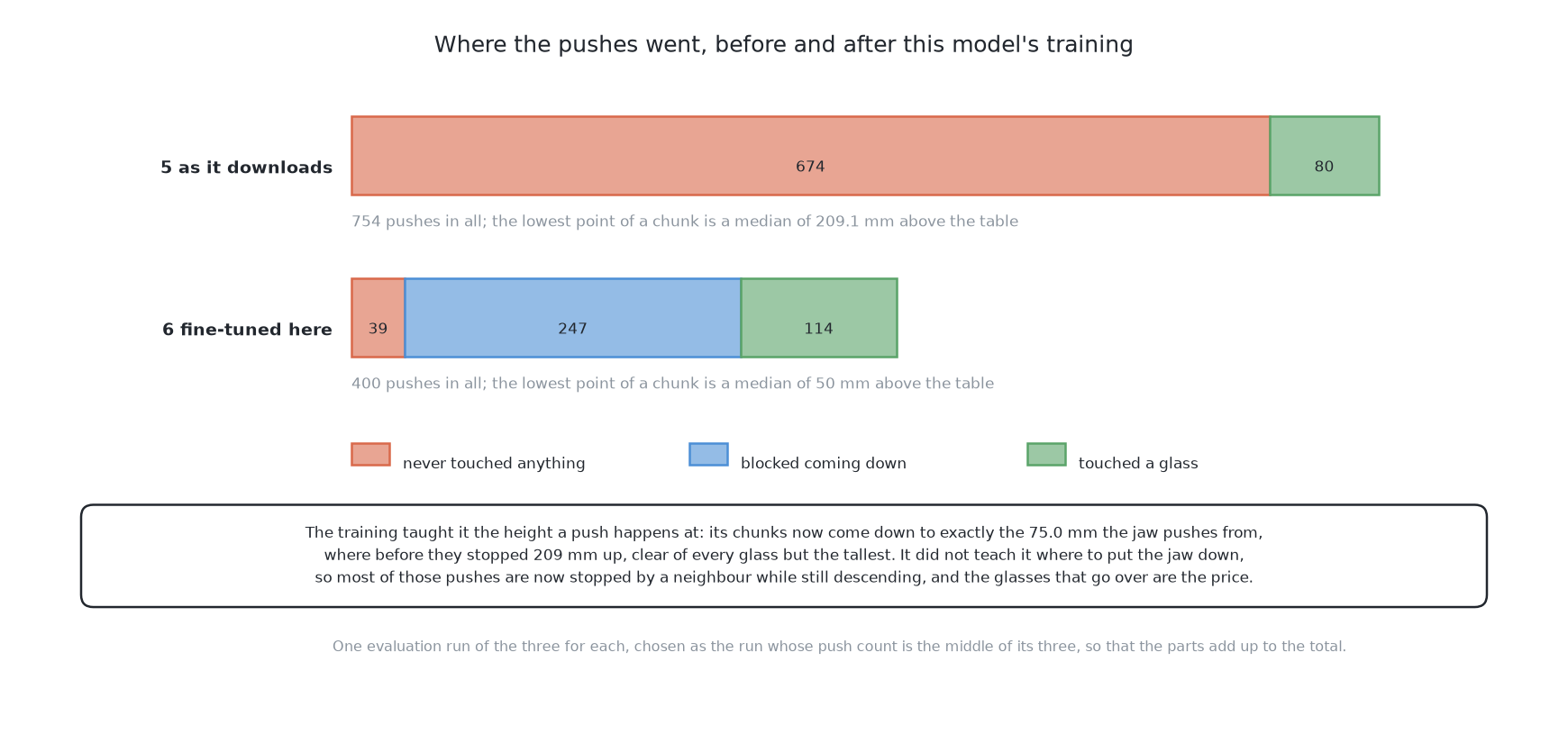
Solution 5 stays out of the wrong column because it never reaches a glass. It hovers, refuses nearly everything, and is marked correct but incomplete. So the gap does not show that training bought nothing. It shows that training bought enough skill to act, but not enough to act safely. A toppled glass cannot be undone. So a policy that does nothing scores better than a policy that does the wrong thing. Any reading of this pair must keep that sentence.
The verdict on the method is still open. More demonstrations have now been tried, and they changed nothing, as the next section shows. Two things are still untried. One is more training steps, because this run used about one part in three hundred of the recipe's compute. The other is DAgger. "The jaw came down on a glass" is a state the teacher never visits, so these demonstrations cannot teach it.
Against solution 3, the question is borrowing against building. Both learn from the same demonstrations, so the data is held still. Solution 3 trains ACT here from random numbers, owns every number in it, and pays nothing for language. This solution borrows 450 million numbers trained on other robots and adjusts a few. So the pair asks whether general knowledge of robot motion beats a small model trained only on this cell.
Against solution 2, the question is teacher against student. Solution 2 explains its refusals and needs no borrowed weights. It is also the ceiling on the pushes this solution copies. So a large win for this solution would be a question about the teacher's ranker, not a success.
Against solution 1, the question is the cheapest method against the most expensive. Solution 1 is a fixed nudge, and every other solution must beat it. If this solution does not beat it by more than its own spread, the 450 million parameters bought nothing.
Against solution 4, the question is planning against reacting. Solution 4 learns how the table changes and searches over pushes at run time. So it can take a new rule by changing its search, and it pays in computation on every push. This solution holds its whole answer in its weights. It can only change by training again.
On the ladder, this solution is where all the fitting happens on borrowed weights. Solution 5, one step below, is where none of it does. The distance between those two is the most useful single number this book can give. The results set the six measured scores side by side.
These scores came from 1,074 demonstrations. The next section asks whether six and a half times as many would change them.
4. More demonstrations, and a result that did not come back#
The scores above say the model acts but does not act safely. Here pushes cost only simulator time. So the obvious question is whether more of them would help, and it can be measured.
The model was fitted again on the new band. Everything else stayed the same: the model, the correction, the thousand steps and the held-out tables. This time there were three seeds, with one scoring run each.
There are three columns, not two. The first large collection ran over the wrong tables by mistake. It is kept as a control. A control is a run that differs in only one thing. This one holds as much data as the new band, but from the old tables. So it separates how much the model learns from where it learns.
In the table below, each column is one fitting. Each cell is the median over three runs, with the standard deviation in brackets. The standard deviation measures how far the runs spread.
| first band, 800 tables from 0, one seed | 5,200 tables from 0, three seeds (the control) | new band, 5,200 tables from 1,000, three seeds | |
|---|---|---|---|
| Demonstrations | 1,074 | 6,907 | 6,935 |
| Glasses racked, of 251 | 56 (±7.6) | 52 (±3.8) | 53 (±2.1) |
| Glasses refused | 138 (±1.0) | 145 (±0.6) | 137 (±4.5) |
| Glasses toppled | 40 (±5.6) | 40 (±3.6) | 42 (±3.6) |
| Tables wrong, of 50 | 36 (±2.9) | 36 (±2.9) | 36 (±1.5) |
| Pushes blocked on the way down | 227 (±8.9) | 217 (±32) | 229 (±45) |
The three columns come from
results.json,
results-band0.json
and
results-aligned.json.
Six and a half times the data changed nothing that can be measured. Compare the first column with the last. Each change is measured in standard errors of the difference. Racked glasses move by 0.7, toppled glasses by 1.0, wrong tables by 1.1 and blocked pushes by 0.1. None reaches two, the point at which the book calls a difference real. So the honest statement is "no change was detected". It is not "the scores are equal". The results explain this rule.
Two details make this reading stronger. The later columns use three separately trained models, so they include the spread between fits. They are still no worse. And leaving out the teacher's own tables changed nothing either.
The control's one striking result did not come back. On the control, refusals rose from 138 to 145. That is ten standard errors, the largest effect in the whole comparison. On the new band, refusals were 137 again. So the effect came from those particular tables and fits, not from the amount of data. This is why the book never trusts a number from one run.
The control also took 1.07 seconds a push, against 0.39 on the new band. That is not the model. The control shared the one graphics chip with another fit, so its clock measured both.
So the data was not the problem. The model fails because its jaw comes down onto glasses. The teacher never does that. So no demonstration shows how to get out of that state, however many there are. DAgger would show it, because it records the teacher's answer in the states the student reaches.
These results close this chapter's argument. The questions and answers gather the chapter's main points in short form.