This page explains what happens inside this solution, part by part. It follows the code and explains what each part of that code does. The model itself, SmolVLA, is described in solution 5's how it works. This page covers only what the training adds.
Contents#
- Fine-tuning — continuing somebody else's training
- Low-rank adaptation — a small correction instead of a large change
- Where the demonstrations come from, and what they cost
- Whether anything but the training differs
- What fine-tuning closes, and what it cannot touch
- Two ways training on one cell's pushes goes wrong
- A second way — the same fine-tune on a larger model
1. Fine-tuning — continuing somebody else's training#
Fine-tuning is the one thing that separates this solution from solution 5. So it comes first.
Training a network works like this. Show it an example. Compare its answer with the wanted answer. Then move every weight a little in the direction that would have helped. After many examples, the weights give good answers. Training from a random start means the weights begin as noise. Fine-tuning means the weights begin at values that somebody else's training already set. So the training has much less to do.
This needs much less data. Each weight is a number the data has to decide. A weight the data cannot pin down ends up fitted to chance details of the examples. With fine-tuning, most weights already have values that work. The data only has to adjust them.
It also saves time. A model trained on robot motion already knows general things. For example, it knows that a motion is smooth and that a jaw approaches a thing before it touches it. These facts carry over to any robot. A random start would spend much of its training learning them again.
What carries over worst is the top-level judgement of what to do next. The borrowed model learned this in other rooms, with other grippers, on tasks that were mostly not pushing. So the training here has more work to do than usual, but still far less than a random start. Solution 3 tests this from the other side. It trains a policy here from random numbers, on the same demonstrations.
The next section explains the cheap way of doing this training that this solution uses.
2. Low-rank adaptation — a small correction instead of a large change#
Plain fine-tuning moves every weight. On a large model that is expensive. Low-rank adaptation is the cheap way, and this solution uses it.
A layer of a network takes a list of numbers in. It multiplies the list by a table of numbers, and hands a new list out. That table is the layer's weights. Low-rank adaptation leaves every borrowed number as it is, and learns a correction that is added to it. The correction is the same size as the table. But it must be the product of two thin tables. The first squeezes the list down to a few numbers. The second expands those few numbers back to full width. Because the squeeze is narrow, the two thin tables hold far fewer numbers than the table they correct. Here the correction holds about four million numbers, against about 450 million in the model.
A table can be written as a sum of simple patterns. The number of patterns it needs is called its rank. A narrow squeeze forces the correction to use only a few patterns. That is why it is called low-rank.
The gain is memory. For every weight that changes, training must also hold its gradient and the optimiser's running averages. The gradient says which way to move the weight. The running averages keep the moves steady. Together these take several times the size of the model. With low-rank adaptation, only the correction needs them. So the memory needed is the model's size plus a little. For this training that was 1.02 GiB, measured while it ran. It fits on this laptop with nothing rented. For a much larger model, such as π0, the same saving decides whether training fits at all. Solution 5 gives those figures.
The cost is that the model can change less. The correction can only move in a few directions in each table. A change that needs the whole table cannot happen. This does not matter when the new task is close to the old one. This cell is far from the old tasks. Its pictures are rendered, it has one gripper and one motion, and its outcomes were never in the borrowed data. So the gap this pair measures is a lower bound on what fine-tuning could buy. A full fine-tune might do better.
One more property matters for the cost of running it. After training, the two thin tables can be multiplied out and added into the borrowed table. This leaves one table of the original size. So the trained model is exactly as large and as fast as the downloaded one. This solution and solution 5 cost the same to run. No gap in their scores comes from extra computation.
The correction needs examples to learn from. The next section says where they come from.
3. Where the demonstrations come from, and what they cost#
The correction is trained on examples. Here an example is a recorded push, with what was seen next to what was done.
Solution 2 is the teacher. It is run over the training half of the tables, and almost every push it makes becomes a demonstration. The observation is this model's input: the view from the top when the push was chosen, the one instruction, and the arm's pose. The action is the path the jaw really followed. The examiner writes this down on every action. So no person had to draw, label or judge anything.
The demonstrations come from a fixed set of tables, called a band. This solution has used two bands, so each number below says which band it comes from.
The first band was 800 tables, starting at table 0. The teacher took 19 minutes of simulator time on it. It gave 1,074 demonstrations from 430 of those tables. On the other 370 tables it found nothing it could push. The teacher made 2,766 pushes. Of these, 1,663 were the 5 mm test pushes that check whether a glass slides. They belong to the shared tipping check, not to the chooser, so they are not demonstrations. Of the other 1,103 pushes, 29 were thrown away. Thirteen toppled a glass, twelve jammed, three pushed a glass out of the zone, and one was blocked on the way down. The project's README for this solution records these counts. The first result, in how it compares, was fitted on this band.
The band then changed to solution 3's band: 5,200 tables, starting at table 1,000. Solution 3 and this solution are compared as a small model against a large one. That comparison is only about the models if both learn from the same tables. The new band also leaves out tables 0 to 199, where the teacher itself was fitted. These were a quarter of the first band. Solution 3 explains why they must be left out.
The change first went wrong, and tests now guard it. The band's numbers were changed in the code. But the program that starts the collection still passed table 0. So the first large collection ran over tables 0 to 5,199, and nothing looked wrong. The project then made the band a named function. Four tests now check it. They check that the band is solution 3's, that the collection starts where the band says, that no band reaches the held-out tables, and that the two bands do not overlap. The wrong collection was kept. How it compares uses it as a control.
On the new band the teacher gave 6,935 demonstrations from 2,796 of the
5,200 tables. This is six and a half times the first band. The project
records it in
demonstrations/collected.json.
Two facts limit what the model can learn from these recordings. First, the
teacher works from the numbers look() hands over, but the student works from
a picture. So a push that depended on a 1 mm difference in the readings must be
learned from pixels. Second, the jaw's force report arrives after the chunk is
chosen. So it is in the recording, but it is not an input the model can use.
The data is free only because this is a simulator and the teacher is a program. Solution 3 explains this point. On a real arm, collecting demonstrations is usually the most expensive part.
The free data has two costs, and solution 3 explains both in full. Its ceiling is the teacher, because the model only copies solution 2 and nothing scores its own pushes. And dropping the failed pushes thins out the hard cases. Here that thinning is small: on the first band, 29 pushes in 1,103, or 2.6 per cent. So the real problem is that the teacher almost never meets a hard table. The student has never been shown one.
The model cannot make better pushes than the best one in its training set. What it can add is steadiness where the teacher was fragile. For example, the teacher may choose almost at random between two close candidates. Averaging over many tables gives a less random choice. The borrowed weights also add a general sense of how a push moves, which the teacher's macro does not have.
The standard repair for states the teacher never visits is DAgger (dataset aggregation). It is cheap here because the teacher is a program. Solution 3 explains it. It is a plan here, not code.
On the new band, solution 3 learns from the same tables. So between those two the data is held still, and only the borrowing differs. This solution is in two pairs at once, and each pair asks a different question.
The data is held still against solution 3. The next section checks that everything except the training is held still against solution 5.
4. Whether anything but the training differs#
A matched pair is only clean if nothing but the training varies. This section checks that.
Most of the setup is the same for both. They see the same tables, the same readings with the same error, and the same view from the top. Both output a chunk of waypoints. Both are marked by the same scorecard and the same topple check. The instruction is also the same sentence. That was kept on purpose, because better-worded instructions for one model would add a second variable.
At the output there is something that looks like a second change. The model outputs numbers in an action space. Their meaning was fixed by the robots it was first trained on. This cell's jaw is not one of those robots. So the numbers must be read as waypoints for this jaw. Solution 5 sets how they are read. Both solutions use that same reading.
The training does not change the reading. It changes whether the model has ever been asked to use it. Solution 5 has to hope its numbers come out at a sensible scale. This solution was trained on real pushes already written in that reading, so it learns this cell's ranges. That is a property of the trained weights, not a second change. So the pair is a clean measurement. The matched pair in the book on telling the glasses apart needed a longer argument here. Its list of category names was a real second change. Here there is no such separate part.
One thing the reading decides reaches into the physics. A chunk holds fifty waypoints, which is the borrowed model's own number. The examiner uses waypoints at a fixed rate, so a chunk is always two and a half seconds of motion. The teacher's push has a hundred waypoints or more, because the teacher feels forward at 10 mm/s and pushes at 20 mm/s. Fitting that push into fifty waypoints makes the student's jaw move at about 31 mm/s on the tuning tables. Over the training tables the project measures 32 mm/s. So the student makes its teacher's pushes faster, and the jaw hits the glasses harder. The examiner caps a path at the jaw's top speed of 200 mm/s, and a chunk the model invents can reach that cap. There are two other choices. One is to change the chunk length, but that is the model's own. The other is to ask several times in one push, but that spends several pushes from the shared budget. The speed-up does not upset the pair, because solution 5's chunks are also two and a half seconds long.
There is one place where the pair could be unfair. A bad reading hurts solution 5 much more than this solution. This solution's training can adjust to a poor reading, but solution 5 cannot. Then the gap would mix what training bought with what the bad reading cost. So the reading must be chosen as well as possible, recorded with solution 5, and left alone once both have run.
The pair is clean. The next section can now say what the training fixed and what it left as it was.
5. What fine-tuning closes, and what it cannot touch#
The pair is a fair test. So this section goes through solution 5's weaknesses one at a time. For each one, it says whether the training repairs it.
The domain gap closes, and this is the large one. A model used across a domain gap usually does not output nonsense. It outputs smooth, sure, wrong actions. These are worse, because nothing later looks suspicious. Solution 5 describes the gap itself.
The gap has been measured, and it is wide. Before the first training step the correction is zero, so the model is exactly solution 5. Its waypoints are then a median of 331 mm from the teacher's on the tuning tables, and 574 mm at worst. The glass zone is only 320 mm by 360 mm. So the untrained answer is not aimed at the wrong glass. It is a motion somewhere else on the table. After five hundred training steps the median was 107 mm.
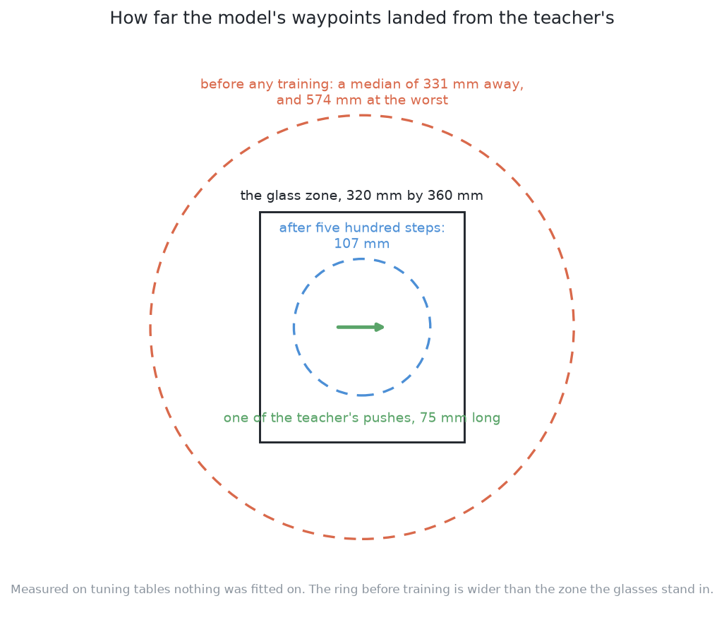
The next five hundred steps cut it again, to 85 mm. These three numbers come from the one fit on the first band. On that fit the error was still falling when the training budget ran out.
That claim did not survive three seeds. A seed is the number that
starts the training's random choices. On the new band the model was fitted
three times, with three seeds. The error at step 500 was 92.6, 115.3 and
77.0 mm. At step 1,000 it was 101.5, 106.1 and 90.0 mm. So it rose in two fits
and fell in one. Between step 500 and step 1,000 the error is flat, inside its
own noise. The fair statement is that the model was not clearly improving at
the end. Each fit records its numbers in its own training file, for example
correction-aligned-0/training.json.
Read every number here as what a thousand steps buys.
Fine-tuning closes the gap because the model is trained on the same kind of input it will be shown. The pale blue glasses, the tan table and the view from the top are now simply what a table looks like to this model.
The scale of the actions is no longer left to chance. This is really two claims, and only one held.
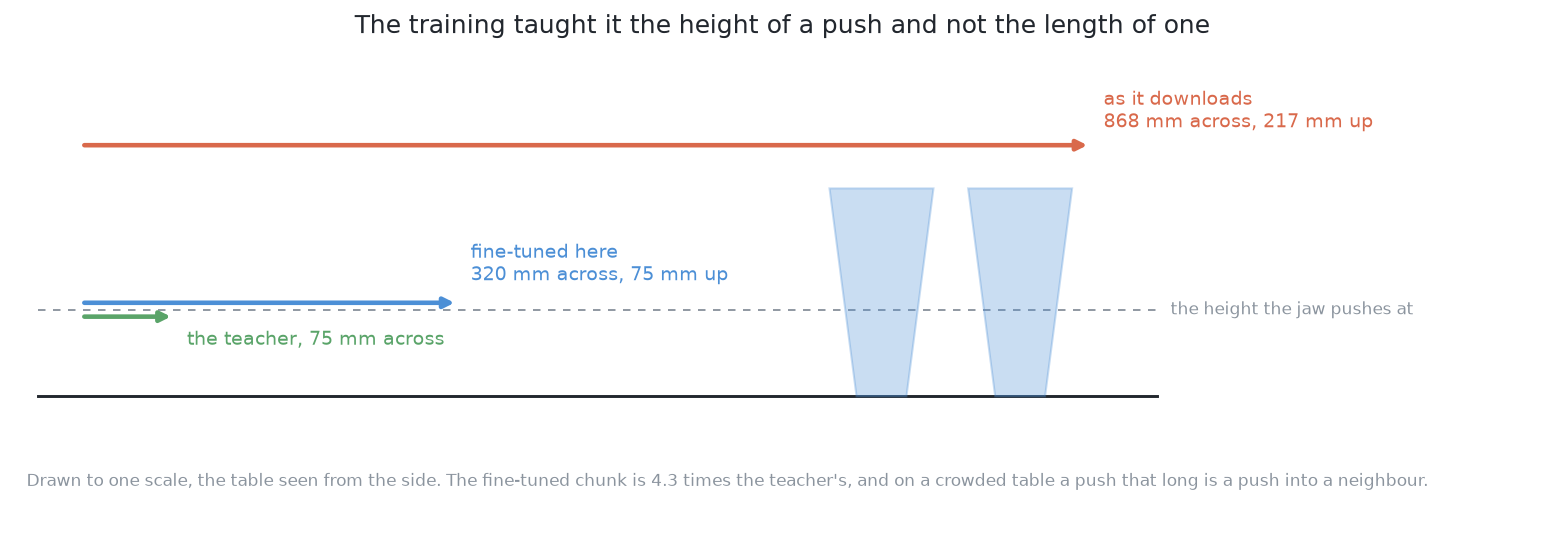
The height was learned. Solution 5's chunks come no lower than 217 mm above the table, so its jaw never reaches the glasses. This model's chunks come down to 75 mm, the height the gripper pushes at. The model learned that a push happens on the table, not above it. This is the clearest sign that the domain gap closed.
The length was not learned. The trained chunks still cover about 320 mm of table. The teacher's pushes on the tuning tables covered 75 mm. The jaw moves at a median of about 92 mm/s, where those demonstrations move at 31 mm/s. This is better than solution 5's 868 mm, but still more than four times too far. A push that is too long, on a crowded table, runs into a neighbour.
Something like friction is stored in the weights, and this needs care. Nobody tells either solution the friction. But the examiner uses the same friction on every table, and every demonstration was made under it. So the trained model can learn how far a glass of this kind goes for a push of this length. No part of it stands for friction. This helps on this examiner and hurts anywhere else. The model holds one fixed value, not a way to measure it. On a table with different friction, the model is wrong with confidence. It is wrong in the direction that topples a glass, because friction also sets the height at which a glass tips.
The weaknesses below survive the training.
The force reading still has no input. The force reading is the only way to observe friction. This model takes a picture, a sentence and the joint readings. Training cannot add a fourth input, as solution 5 explains.
The instruction still carries nothing. It is the same sentence on every table, as solution 5 explains. Training makes this worse. When every example has the same instruction, the model is likely to learn to ignore it. Yet the model still pays for its language part in size and memory. Solution 3 uses a policy with no language part at all.
The refusal still cannot be the policy's. A policy has no place for a rule, so the topple check stays outside it, in pushing without toppling. Training makes one thing worse. The teacher refused the glasses it should refuse, so the training set has no example of a glass that must not be pushed. The policy proposes a push on such a glass as readily as on any other, and the shared check stops it.
It still cannot explain a refusal. Solution 2 can print why a glass tips. A policy that was stopped has nothing to say.
A surprise in the middle of a chunk is still carried out. The model commits to a whole chunk, as solution 3 explains. Training changes how often a surprise comes. It does not change what happens when one does. The early abort that would read the force during a push is a design, not code. The examiner only stops at a jam. This is the same for both solutions, so it does not upset the pair.
The run-time cost is the same, because the correction folds into the weights. The input's error is also the same. No training makes a reading more accurate. Training can only help the policy cope when a reading is a little wrong.
The training fixes some things. The next section names two ways the training itself can go wrong.
6. Two ways training on one cell's pushes goes wrong#
Training helps, but it also has risks. Two of them have names.
Catastrophic forgetting. Training on a narrow set of examples moves the weights away from what they knew before. The model gets better at this cell and worse everywhere else. Low-rank adaptation softens this, because the borrowed numbers are never overwritten. The correction can be removed to get the original model back. But the corrected model is the one that runs, and it would be poor on any other robot. Here that is not a loss, because the model only ever sees this examiner's tables. But the correction must be kept in step with the cell.
Overfitting. A model trained on few examples can learn the examples instead of the skill. Here that would mean learning the tables instead of the pushing. The examiner guards against this. It never marks a solution on a table it trained on. And demonstrations cost only simulator time, so the training set can be large.
The two risks pull against the gain. More training closes the domain gap further, but it also makes both risks more likely. So there is a right amount of training, not a maximum, and the held-out tables decide it. Here, between step 500 and step 1,000, the training loss halved. On the first fit, the error on the tuning tables fell by only about a fifth, from 107 mm to 85 mm. On the three later fits it did not fall at all, as the domain gap paragraph shows.
There is one more thing to know. The policy is random: asked the same question twice, it may act differently. Training also depends on its random seed. So the examiner asks for several training seeds and several runs. The first fit used one seed. The re-fit on the new band used three. This matters most here, because the thing measured is a gap between two solutions. A gap smaller than either solution's own spread has not been shown to exist.
These risks are about one model. The next section asks whether a larger model would do better.
7. A second way — the same fine-tune on a larger model#
The sections above use one model, SmolVLA. One model cannot say whether a much larger one would do better. The second way is the same fine-tune on π0.5. It uses the same demonstrations, the same low-rank adaptation and the same examiner, with a much larger model. Only the model changes, so the gap would measure what size is worth. The library already includes π0.5, so the same training code can point at different weights.
It is not built, because most mistakes are in the pipeline, not the model. Rendering the view, recording demonstrations, reading the actions and running the evaluation all break in ways found only by a failed run. SmolVLA runs on a laptop, so those failures cost nothing. On the large model, each failed run would use rented time. A weekend of rented time costs about a hundred dollars, and could produce no comparison at all.
The question is now asked with a different model. Solution 7 fits Evo-1, a newer and larger model that runs on this laptop. It used the same 6,935 demonstrations and the same thousand steps, with three seeds. It did not learn the task, while this solution's fits on the same data did. Solution 7's results give the numbers, and say why this does not show that the newer model is worse.
← The code · A worked example →