This page answers one question. You have downloaded a model that someone else trained, and it almost does what your robot needs, so how do you teach it the last part using only a small amount of your own data?
The page explains the three usual ways to do this, and they differ mainly in how much of the model you allow training to change. You can freeze most of the model and train only a new last layer, or you can add a small side path called LoRA and train only that, or you can train every number in the model. For each of the three the page says how much data and how much memory it needs, what the model can forget along the way, and how to choose between them.
It is for a reader who has read the chapter so far, because it uses words that the earlier pages introduced. You should know what a layer, a backbone, a head and a parameter are, from inside a neural network. You should also know what pretraining is, from where the data comes from. That page introduced fine-tuning in a single section, whereas this page goes inside it and explains how the work is actually done.
Contents#
- The idea in one sentence
- Three ways to fine-tune
- LoRA in plain words, with real counts
- A worked example: 50 examples, four ways
- Forgetting
- How much data and how much memory
- Two examples on a robot arm
- Where it works and where it does not
- Libraries and scripts
- How to choose, and what each way costs
- Where to read next
- Using it in Python
1. The idea in one sentence#
Fine-tuning means taking a model that was already trained on a large, general pile of data, and training it a little more on a small pile of your own data, so that it does your job.
Here is an everyday example. When an experienced lorry driver joins a new company, the driver does not relearn how to steer or brake, and instead learns only the new routes and where the loading bays are. In the same way a pretrained seeing model already knows about edges, surfaces and shapes, so it only needs to learn what your own parts look like.
The model you start from is called the pretrained model. Its numbers are the pretrained weights. Most pretrained models are split into a backbone, the large first part that turns the input into useful numbers, and a head, the small last part that turns those numbers into the answer. The seeing models overview describes this split for pictures.
2. Three ways to fine-tune#
The three ways differ in which numbers training is allowed to change, and that single difference is what decides their cost. A number that training may not change is called frozen.
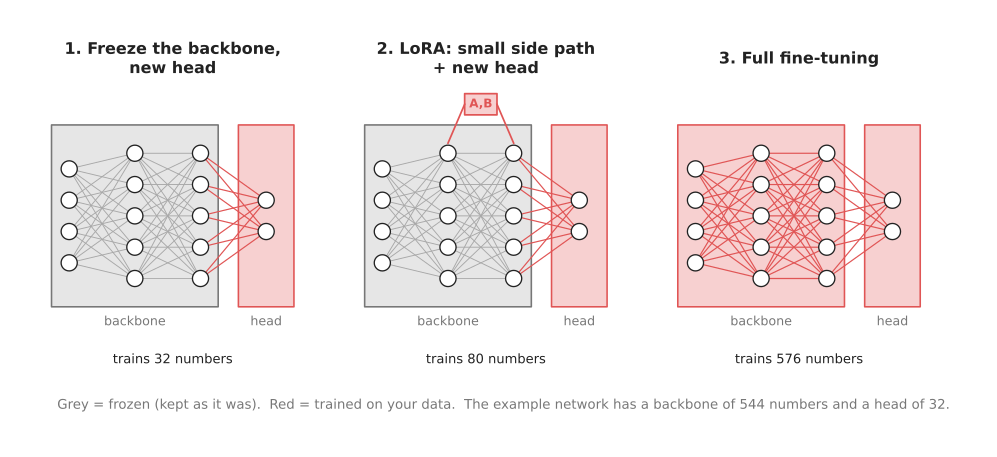
Grey parts are frozen and red parts are trained. The counts under each network are for the small network of the worked example in section 4.
Way 1: freeze the backbone and train a new head. You keep every number in the backbone exactly as it was, and then you throw away the old head and put a new, small head in its place, so that only the new head is trained. People also call this a linear probe when the new head is a single layer. It is the cheapest of the three ways, because so few numbers change, and it works whenever the backbone already turns your pictures into numbers that separate your answers well.
Way 2: add a small side path and train only that. You keep every original number frozen, but you add a few small extra layers next to or inside the old ones, and then train only those together with a new head. These extra layers are called adapters, and the most used kind of adapter is LoRA, which stands for low-rank adaptation and is explained in section 3. This way is useful because it lets the backbone's behaviour change a little while still training very few numbers.
Way 3: full fine-tuning. Every number in the model may change, which makes this the most flexible of the three ways. However that flexibility has a price, because it needs the most memory and it is the most likely to forget what the model knew before.
There are mixtures of these three ways as well, and a common one is to freeze the first layers of the backbone while training all the rest. This works because the first layers find edges and colours, which look the same for every job, so they rarely need to change at all.
3. LoRA in plain words, with real counts#
A layer in a network holds its weights in a grid of numbers. A layer that turns 4,096 numbers into 4,096 numbers has a grid of 4,096 rows and 4,096 columns. That is 16,777,216 numbers. The large language models inside vision-language-action models, such as the one inside OpenVLA, are built from many layers of about this size.
Full fine-tuning would change all 16,777,216 numbers in this one grid, whereas LoRA leaves the grid frozen and adds a separate change to it, building that change from two thin grids multiplied together.
- Grid A has a few rows and 4,096 columns.
- Grid B has 4,096 rows and a few columns.
- B multiplied by A gives a full 4,096 by 4,096 grid of changes.
The "few" is called the rank, so a rank of 32 means that grid A has 32 rows and grid B has 32 columns. Together the two thin grids then hold 32 x (4,096 + 4,096) = 262,144 numbers, which is only 1.56 % of the full grid. The layer works out its answer using the frozen grid plus the change, which means the original numbers are never touched.
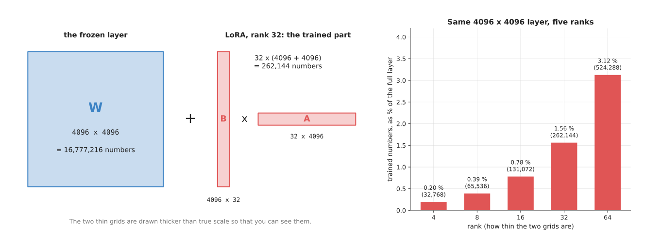
The left side shows the frozen grid and the two thin grids that LoRA trains. The bar chart shows how the trained share grows with the rank, for the same layer.
The table below lists the numbers from the bar chart. Read each row as: the rank, how many numbers LoRA trains for this one layer, and what share of the full grid that is.
| Rank | Numbers LoRA trains | Share of the full 16,777,216 |
|---|---|---|
| 4 | 32,768 | 0.20 % |
| 8 | 65,536 | 0.39 % |
| 16 | 131,072 | 0.78 % |
| 32 | 262,144 | 1.56 % |
| 64 | 524,288 | 3.12 % |
Why does such a thin change work? The authors of LoRA found that the change which fine-tuning makes to a large pretrained model usually has a simple shape, and a simple change can be written well with only two thin grids. You do lose a little flexibility this way, but in return you train and store far fewer numbers.
LoRA has two further benefits on a robot. First, because the side path is a small separate file, you can keep one pretrained model together with several small LoRA files, one for each task, and load only the one you need. Second, you can switch the side path off, and the model is then exactly the pretrained model again.
OpenVLA's own LoRA script uses a rank of 32 and adds LoRA to every fully connected layer. The LoRA paper reports that, for the 175-billion-parameter language model GPT-3, LoRA cut the number of trained numbers by 10,000 times and the graphics card memory by 3 times, compared with full fine-tuning.
4. A worked example: 50 examples, four ways#
This example is a real run in numpy, in the diagram script
models_extras.py. The network is tiny, so that
the run takes seconds, but the steps are the same as for a large model.
The set-up is this.
- A "pretrained" network reads 16 numbers. Its backbone has one layer of 32 neurons, which is 544 numbers. Its old head gives 4 answers for an old job.
- The new job needs 1 answer. It uses features close to, but not the same as, the ones the backbone already makes. In the script, the new job is built from the same backbone with a small change added.
- There are only 50 examples of the new job to learn from. That is like having 50 demonstrations of a new task.
- The network is trained four ways, for 3,000 steps each, and tested on 2,000 new examples it never saw.
The error is the mean squared error, which is the average of the squared difference between the answer and the right answer, so a lower number is better. To give the numbers a scale, a model that always guessed the average answer would score 0.487.
The table below gives the result. Read each row as one way of training: how many numbers it trained, its error on the new job, and its error on the old job afterwards.
| Way | Numbers trained | Error on the new job | Error on the old job afterwards |
|---|---|---|---|
| Freeze the backbone, new head | 32 | 0.041 | 0.000 |
| LoRA, rank 1, plus a new head | 80 | 0.045 | 0.049 with the side path on, 0.000 with it off |
| Full fine-tuning | 576 | 0.069 | 0.098 |
| From scratch, with no pretraining | 576 | 0.172 | not meaningful |
Four things show up.
- Starting from pretrained weights matters most. All three fine-tuning ways beat training from scratch by a wide margin. From scratch, 50 examples are not enough to learn good features.
- With little data, training fewer numbers did better. Full fine-tuning learned the 50 examples perfectly, with a training error of 0.000, and still did worse on new examples than the two cheaper ways. It had enough freedom to learn the examples' noise as well as their pattern. This is called overfitting, as how a model learns explains.
- Here the new job was close to the old one. So a new head on the frozen backbone was enough, and it did slightly better than LoRA. When the new job needs features the backbone does not make, the head alone cannot fit it, and LoRA or full fine-tuning pulls ahead.
- Full fine-tuning damaged the old job. The next section is about this.
This is only one small run, so with another set-up the order of the first three rows can change. However the first and the last of the four points above hold in general.
5. Forgetting#
When full fine-tuning changes the backbone, it also changes the features that the old head relied on, so the old job gets worse. This is called catastrophic forgetting, although the word "catastrophic" is historical and the loss is often only partial, as it is here.
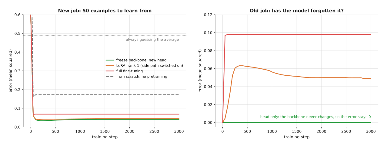
The left panel shows the error on the new job during training. The right panel shows the error on the old job during the same training.
On the right, the green line stays at 0, because freezing the backbone means the old job's features cannot change at all. The red line jumps to 0.098 within 50 steps, which shows that full fine-tuning bent the backbone towards the new job straight away. The orange line is LoRA with its side path switched on, and it damages the old job too, by 0.049. However switching that side path off gives back the pretrained model exactly, with an error of 0.000.
Forgetting matters on a robot in two places.
- A vision-language-action model fine-tuned on your task can lose some of its general knowledge of objects and words, so it may follow your task well and then fail on a new instruction it would once have understood. The vision-language-action page describes how laboratories mix general data into training to reduce this.
- A detector fine-tuned only on your five parts can stop finding people and hands, if it once found them, so if a safety check depends on those classes you should keep a separate model for them.
There are four usual defences against forgetting, and they can be combined. You can freeze more of the model, so that fewer of the old features are able to move. You can use LoRA and keep the pretrained model beside it, because the side path can then be switched off. You can mix some of the original kind of data into your fine-tuning data, so that the old job is still being practised. Finally you can train for fewer steps with a small learning rate, which is the size of each step in training.
6. How much data and how much memory#
Data#
The amount of data depends more on how far your job is from the pretrained job than on the way you fine-tune. The table below gives the usual ranges already quoted in this book. Read each row as: the kind of model, and how much of your own data people usually start with.
| Kind of model | Usual amount of your own data | Where this book says so |
|---|---|---|
| Detector for your parts | a few hundred labelled pictures; 80 drawn pictures in a simple case | object detection, Book 2's worked example |
| Vision-language-action model for a new task | tens to hundreds of demonstrations | vision-language-action models |
When your data is at the small end of these ranges you should freeze more of the model, whereas at the large end you can afford to train more of it.
Memory#
Training needs far more memory than running a model. The graphics card must hold the model's weights. For every trained number it must also hold that number's gradient, which says which way to change it, and the extra numbers the optimiser keeps. The optimiser is the part of the training program that makes the changes. A widely used optimiser called Adam keeps two extra numbers for every trained number.
A rough count shows why full fine-tuning is so expensive. A common figure is about 16 bytes of memory per trained number, when training with Adam and a mix of 16-bit and 32-bit numbers. OpenVLA has about 7 billion parameters. Full fine-tuning would need about 7 billion x 16 bytes = 112 GB, before any pictures are loaded. No single graphics card holds that. With LoRA, only 1 % to 2 % of the numbers are trained, so the gradients and optimiser numbers become small. The frozen weights still have to be held. At 2 bytes each, 7 billion weights take about 14 GB.
The real figures come from the projects themselves. Book 3 collects the openpi figures in working without a GPU, and the OpenVLA README gives its own.
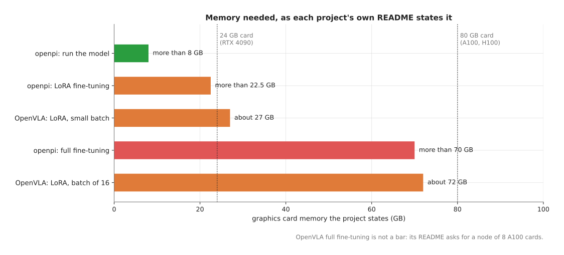
Each bar is a figure that a project states in its own README, and the two dotted lines are common graphics card sizes, so you can see at a glance which jobs fit on which card.
The table below gives the same figures. Read each row as: the project, what you want to do, and the memory its README states.
| Project | Job | Memory stated |
|---|---|---|
| openpi (π0 and π0.5) | run the model | more than 8 GB |
| openpi | LoRA fine-tuning | more than 22.5 GB |
| openpi | full fine-tuning | more than 70 GB |
| OpenVLA | LoRA fine-tuning, smaller batch | at least about 27 GB |
| OpenVLA | LoRA fine-tuning, batch of 16 | about 72 GB |
| OpenVLA | full fine-tuning | a full node of 8 A100 cards |
A batch is the number of examples the training program looks at before it makes one change, and a smaller batch needs less memory, which is why OpenVLA's LoRA figure appears as two separate rows.
For a detector, memory is rarely the problem at all, because a small YOLO model fine-tunes on an ordinary processor with no graphics card whatsoever, as the Book 2 example shows.
7. Two examples on a robot arm#
Fine-tuning a detector on your parts#
A cell sorts five kinds of machined bracket off a conveyor, however a detector trained on the COCO photo collection knows about cups and bottles and has never seen a bracket.
- Take a few hundred pictures of the brackets with the robot's own camera, in the cell's own light, with the parts in many positions.
- Draw a box around each bracket and give it one of five names.
- Start from a pretrained YOLO model and train it on these pictures. The backbone
is not frozen by default in Ultralytics, so this is full fine-tuning of a small
model. Ultralytics'
freezetraining option freezes the first layers if you have very few pictures. - Test on pictures the model never saw, including awkward ones: parts touching, parts half out of the picture, the light turned down.
This works well because the new job is close to the pretrained job, since finding objects is the same skill either way and only the names and the shapes are new.
Fine-tuning a vision-language-action model on 50 demonstrations#
A lab wants a vision-language-action model to put a cup on a saucer, on its own arm.
- Record 50 demonstrations. A person drives the arm through the task with a leader arm or a hand controller, and the robot records the camera pictures, the joint angles and the instruction "put the cup on the saucer". The page where the data comes from describes recording.
- Convert the recordings into the format that the model's scripts expect. openpi reads the LeRobot dataset format, and OpenVLA reads a format called RLDS.
- Run LoRA fine-tuning. This fits the memory of one rented card, as the Book 3 cost section works out.
- Test on the real arm, with the cup in places the demonstrations did not use. Count successes out of, say, 20 tries.
Fifty demonstrations is at the small end of the usual range, so it can be enough as long as the scene stays much like the demonstrations themselves. If the model fails once the cup moves, then the usual fix is more demonstrations with more variety in them, rather than a different way of fine-tuning.
8. Where it works and where it does not#
The two examples above both worked, so it is worth saying plainly when fine-tuning does not. Fine-tuning works when the new job is close to what the model was pretrained on, which is why a detector pretrained on everyday photos adapts well to parts on a table: both are colour pictures of solid objects.
There is also a case where fine-tuning is the wrong shape of answer rather than a failing one. The cost of this page is paid once for each task, so a robot asked to do twenty different jobs pays it twenty times, and a robot whose jobs change every week pays it every week. Prompting with a demonstration is the alternative in that situation: the model is left alone and is shown one recording of the task instead. It is less accurate on any single task, for a reason that page measures, and today no model that works this way can be downloaded.
It works badly in the cases below, and the table gives each one together with the sign you would see and what people do instead.
| When it goes wrong | The sign you would see | What people do instead |
|---|---|---|
| The new data looks nothing like the pretraining data, such as depth images or X-rays given to a colour-photo model | even full fine-tuning gives poor test results | pick a model pretrained on similar data, or collect much more data |
| Too little data for the number of trained numbers | training error near 0, test error high | freeze more, use LoRA with a small rank, or collect more data |
| Your test pictures are too like your training pictures | good scores in testing, failures in the real cell | test on pictures from another day, another light and new part positions |
| The model forgets something it needs | a class or a skill that used to work now fails | LoRA with the side path kept separate, or mix in general data |
| The labels are inconsistent | the model is unsure in exactly the cases where people disagreed | fix the labels; no training method fixes them for you |
9. Libraries and scripts#
These are all real tools that you can download today, and each one is named below together with what it does for you.
- Hugging Face PEFT is a Python library
for "parameter-efficient fine-tuning", which means training a small part of a model.
You describe the adapter with
LoraConfig, wrap the model withget_peft_model, andprint_trainable_parameters()then tells you how many numbers will be trained. OpenVLA's LoRA script is built on it. - OpenVLA ships
vla-scripts/finetune.pyfor LoRA fine-tuning, andvla-scripts/train.pyfor full fine-tuning across several cards. Its README now also points to a newer recipe, called OFT, for better results. - openpi fine-tunes the π0 and
π0.5 models. You first run
scripts/compute_norm_stats.py, which measures the range of your robot's numbers, and thenscripts/train.pywith a training configuration. Its original version uses the JAX library, whereas its newer PyTorch version does not yet support LoRA training. - Ultralytics fine-tunes YOLO
detectors with one call,
model.train(...). Itsfreezeoption freezes the first layers. Book 2 has a complete worked example. - LeRobot trains and fine-tunes smaller robot policies, such as SmolVLA and ACT, and runs on a Mac.
10. How to choose, and what each way costs#
Start with the cheapest way that could work, and move to the next only if the results show you need it.
- Freeze the backbone and train a new head when your data is small and your job is close to the pretrained job. It is fast, it cannot forget, and it needs little memory. It costs you flexibility: if the backbone's features do not separate your answers, no head can fix it.
- Use LoRA or another adapter when a new head is not enough, or when the model is too big to fully fine-tune on the card you have. For vision-language-action models, this is the usual first choice. It costs you a little accuracy compared with full fine-tuning on large data, and a few extra settings to choose, such as the rank.
- Fully fine-tune when you have plenty of data, the job is far from the pretrained job, and you have the memory. For small detectors, this is the normal choice, because the model is small. It costs you memory, time, and the risk of forgetting.
The obvious alternative to all three is to train a model from scratch on your own data. The worked example shows why people rarely do: with 50 examples, the model trained from scratch had an error of 0.172, against 0.041 to 0.069 for the three fine-tuning ways. Pretraining gives you knowledge that your small dataset could never teach. Training from scratch only makes sense when no pretrained model has seen anything like your data, and you have a very large amount of it.
The cost of fine-tuning in general is the data you collect and label, the graphics card time, and the testing. The testing is the part that people most often skip, and the part that decides whether the robot works.
11. Where to read next#
- Running a model on a robot is the next page. It covers what changes once the fine-tuned model runs on the arm.
- Classical machine learning covers smaller models that are not neural networks, which sometimes need no fine-tuning at all.
- Prompting with a demonstration is the alternative to this whole page, in which the model never changes and the task arrives as a recording.
- Uncertainty and confidence explains how to tell when a fine-tuned model is sure and wrong.
- Object detection explains the detectors that you would fine-tune on your parts.
- Vision-language-action models explains the models that are fine-tuned on demonstrations.
- Working without a GPU in Book 3 says what training you can do on your own computer, and what it costs to rent a machine for the rest.
12. Using it in Python#
Section 3 explained LoRA as two thin grids, and section 9 named the library that inserts them. This section puts the two together, so that after reading it you will know that "use LoRA" means writing one configuration object and one wrapping call, and that you never touch the thin grids yourself.
import torch
from peft import LoraConfig, get_peft_model
from transformers import AutoModelForVision2Seq

vla = AutoModelForVision2Seq.from_pretrained(
    'openvla/openvla-7b', torch_dtype=torch.bfloat16, trust_remote_code=True)

config = LoraConfig(
    r=32,                          # the rank of section 3
    lora_alpha=16,                 # how strongly the side path is added on
    lora_dropout=0.0,
    target_modules='all-linear',   # a side path on every fully connected layer
    init_lora_weights='gaussian',
)
vla = get_peft_model(vla, config)
vla.print_trainable_parameters()   # how many numbers will really be trained
Those are the settings OpenVLA's own vla-scripts/finetune.py uses, so the numbers in
the table in section 3 are the numbers this code produces. Training then runs as
normal, and when it finishes vla.save_pretrained('my-adapter') writes only the side
paths, which is why an adapter is a few megabytes rather than a few gigabytes.
PEFT gives you the whole of way 2. get_peft_model walks through the model, replaces
every layer that target_modules matches with a version that has the two thin grids
beside it, and freezes everything else, so the "1 % to 2 % of the numbers" in section 6
happens without your counting anything. print_trainable_parameters prints that count,
and it is worth reading every time, because a target_modules setting that matches
nothing fails silently and trains nothing at all.
What you have to collect yourself is the data, and that is the part that takes weeks rather than minutes. You record the demonstrations, and you convert them into the format the project's scripts read, which is the LeRobot dataset format for openpi and RLDS for OpenVLA, as section 7 describes. You also have to write the training loop, or else use the project's script, because PEFT only prepares the model and does not train it.
What you have to decide is the rank, which layers get a side path, and how long to
train. Start with the rank and the settings above, because they are what the model's
authors used, and change the rank only when the results in section 10 tell you to.
Fine-tuning a detector needs none of this, because the whole job is a single call:
YOLO('yolo11n.pt').train(data='parts.yaml', epochs=100, imgsz=640, freeze=10), where
freeze=10 keeps the first ten layers fixed for the case where you have very few
pictures.