A learned model can look good on a computer and still fail on an arm. This page answers one question: how do you tell whether a model is good enough to run on a real arm, and what should the arm do on the runs where it is not?
It is for a beginner who has read the earlier pages of this chapter, especially running a model on a robot and fine-tuning, because it uses the words those pages introduced. It covers test sets and real trials, how many trials you need, what to write down on every trial, how to sort failures, how the arm should behave when it fails, and finally how to move a model from simulation to the real arm.
Every number on this page comes from a real run of the diagram script
making_models_work.py, and the
confidence intervals in it are computed exactly from the binomial distribution. The
only exception is the trial log in the worked example, which is a made-up example,
and the page says so again where it is used.
Contents#
- The idea in one sentence
- A test set is not a trial
- Counting successes, and how sure the count is
- Running fair trials
- What to log on every trial
- Sorting failures into kinds
- What the arm should do when it fails
- From simulation to the real arm
- A worked example: a mug-picking model, from test set to 100 trials
- Where it is used on a robot arm
- What goes wrong, and what people do about it
- Libraries and tools
- Why this rather than the obvious alternative, and what it costs
- Where to read next
- Using it in Python
1. The idea in one sentence#
A model is good enough for an arm when it succeeds often enough in real trials, counted over enough trials to be sure of the number, and when the arm does something safe on the trials where it fails.
Here is an everyday example. A new driver who passes a written test knows the rules, however you only learn whether they can actually drive by watching them drive many times on different roads. You also want to know what they do when something goes wrong, which the written test never shows you.
2. A test set is not a trial#
A test set is a set of examples that the model did not train on. You run the model on them and compare its answers with the right answers. The how a model learns page explains why these examples must be kept back from training.
A trial, by contrast, is one real attempt at the whole job on the arm, such as starting with a mug on a rack and ending with that mug on a tray. A trial either succeeds or fails outright, and the success rate is simply the share of trials that succeed.
A test set score is quick and cheap, so it is still worth having, because it catches a broken model before it ever goes near the arm. However it answers a different question from the one you care about, and there are three reasons why it does not predict the success rate.
- The test set checks single steps, whereas a trial is many steps in a row. A movement model decides a new action many times a second, so a tiny mistake on one step moves the arm a little off course, which means the next picture is one the model has never seen. The behaviour cloning page calls this compounding error.
- The test set measures closeness to a person's answer rather than success. A grasp 1 cm away from the one in the demonstration counts as an error on the test set, and yet on the arm it may work perfectly well. The reverse also happens, because a grasp that is very close to the demonstration may still let the mug slip.
- The test set was recorded on another day. The light, the camera position and the objects in real trials are never quite the same.
The picture below shows that first reason with simple numbers. Suppose each step of a trial is right with some fixed chance, and suppose any single wrong step spoils the whole trial, so that a trial of N steps is clean only with that chance multiplied by itself N times.
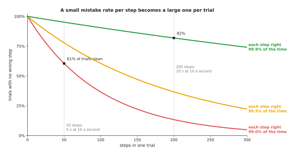
Read each curve as one model. The red model is right on 99% of steps, which sounds very good indeed. However at 10 decisions a second a 5-second trial has 50 steps, so only 60.5% of its trials are clean, and a 20-second trial has 200 steps, where only 13.4% are clean. Even the green model, which is right on 99.9% of steps, has only 81.9% clean trials at 200 steps.
Real trials are kinder than this arithmetic suggests, because a good policy often recovers from a small mistake and many wrong steps do no harm at all. The curves are therefore a warning rather than a forecast, and the point they make is that a per-step score can look almost perfect while the trial success rate is poor. The only way to know the success rate is to run real trials.
3. Counting successes, and how sure the count is#
Say a model succeeds in 18 of 20 trials, which gives a success rate of 90%. However if you ran 20 more trials you might see 16, or you might see 20, so the true success rate, meaning the one you would see over thousands of trials, is somewhere near 90% without your knowing exactly where.
A confidence interval gives the range. A 95% confidence interval is a range worked out so that, if you repeated the whole experiment many times, the range would contain the true rate 95 times in 100. The standard one for a count of successes is the Clopper-Pearson interval, which is also called the exact interval. You do not need its formula at all, because a library computes it in one line, as section 12 shows.
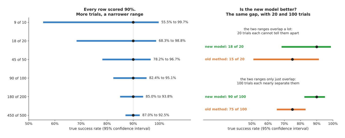
The left half of the picture shows what the number of trials does, and every row in it scored exactly 90%. The table below gives the same ranges as numbers, so read each row as one experiment.
| Successes | Success rate | 95% confidence interval |
|---|---|---|
| 9 of 10 | 90% | 55.5% to 99.7% |
| 18 of 20 | 90% | 68.3% to 98.8% |
| 45 of 50 | 90% | 78.2% to 96.7% |
| 90 of 100 | 90% | 82.4% to 95.1% |
| 180 of 200 | 90% | 85.0% to 93.8% |
| 450 of 500 | 90% | 87.0% to 92.5% |
So 18 of 20 only tells you that the model is somewhere between fairly poor and nearly perfect, whereas 90 of 100 tells you it is somewhere between 82% and 95%. To halve the width of the range you need about four times as many trials.
The right half shows the question people usually ask, which is whether the new model is better than the old method. With 20 trials each, 18 against 15 looks like a clear win, however the two ranges of 68.3% to 98.8% and 50.9% to 91.3% overlap a great deal. With 100 trials each, 90 against 75, the ranges become 82.4% to 95.1% and 65.3% to 83.1%, so they only just overlap, and that is the point at which the difference starts to be real.
Two more cases come up often.
- No failures at all. If a model succeeds in 20 of 20 trials, then the true failure rate could still be as high as 16.8%. A quick rule called the rule of three says that with no failures in N trials the failure rate is probably below 3 / N, so for 20 trials that gives 15%, which is close to the exact 16.8%, and for 300 trials it gives 1%.
- Two close methods. Checking that two ranges do not overlap is a simple but rough test, so for a close comparison you should run both methods on the same list of starting setups and compare them setup by setup, which is called a paired comparison.
Book 3's simulation and evaluation page makes the same point about research papers, because it shows that 20 of 25 and 19 of 25, as papers often report, cannot be told apart at all, and it describes the benchmarks and the efforts to fix them. This page does not repeat any of that, since it is about your own model on your own arm.
4. Running fair trials#
Since the number of trials decides how much the success rate tells you, the next question is how those trials are run. A success rate means something only if the trials were fair, and the six rules below are what make them fair.
- Write down what success means before you start. For example: "the mug is upright on the tray within 30 seconds, and nothing was touched except the mug". Deciding afterwards lets you count a near miss as a success without noticing.
- Fix a list of starting setups. Write down, or photograph, where the mug and the other objects start in each trial. Cover the range the arm will really meet: different positions, turns, mugs and lighting. Then use the same list for every model you compare.
- Mix the order. Do not run all trials of the old method in the morning and all trials of the new model in the afternoon, when the light has changed. Take turns.
- Use the same time limit for every trial, and count a trial that runs out of time as a failure.
- Do not stop early because the numbers look good. Decide the number of trials first. Stopping as soon as the rate looks high picks a lucky moment.
- If you can, let the person who judges success not know which model ran. This is called a blind trial. It stops the judge from being kinder to the model they hope wins.
5. What to log on every trial#
Fair trials give you a success rate, which tells you how often the model fails, whereas a log is what tells you why it failed. Record the things below on every trial, including the successes, because a success that nearly failed is a warning as well.
| What to log | Why |
|---|---|
| the model's name and version, and the settings it ran with | so you know exactly which model scored the number |
| the starting setup, as a photograph and a number from your list | so you can run the same setup again |
| every camera picture, or at least a few per second | so you can see what the model saw when it went wrong |
| every action the model gave, and the time it took to answer | so you can find the step where it went wrong, and spot slow answers |
| the joint positions, and the gripper's opening and force | so you can tell a slip from a missed grasp |
| the model's confidence, if it gives one | so you can check whether low confidence came before failure |
| every safety check that fired, and every time a person stepped in | these are failures, even if the trial ended well |
| the result, the time taken, and a short note from the person watching | the note is often the fastest way to sort the failure |
This is more data than it sounds, because a few minutes of pictures from two cameras can come to hundreds of megabytes. Keep it anyway, since a failure you cannot replay is a failure you can only guess about. The tools in section 12 store it in standard formats.
6. Sorting failures into kinds#
Once you have a log for every trial, you can use it to sort the failures. After a batch of trials, go through every failure and give it exactly one kind, where the useful kinds are named after the part of the system that went wrong, such as seeing, grasping, the movement policy, safety or time. Then count how many of each kind you have.
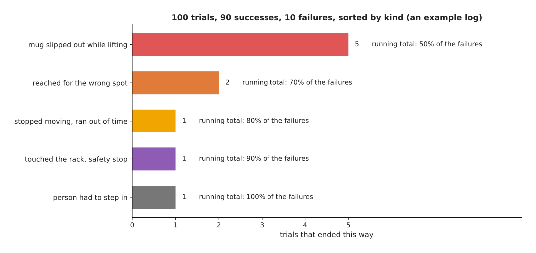
The counts in this picture are a made-up example. They show a pattern that is common in practice. One kind of failure, here the mug slipping out while lifting, causes half of all failures. The top two kinds cause 70%.
Sorting pays off in three ways.
- It tells you what to fix first. Fixing the slips could remove half of the failures, whereas fixing the one timeout would remove only a tenth of them.
- It tells you whether a model is the problem at all. A slip may come from the gripper's force rather than from the model, and a wrong spot may come from a camera that has moved and needs calibration again.
- It tells you what data to collect. If most failures are slips, the next demonstrations should include lifts that almost slip and are caught. The fine-tuning page shows how to train on them.
After making a fix, run the same list of setups again and sort the failures again, because a fix often moves failures from one kind to another instead of removing them.
7. What the arm should do when it fails#
Sorting failures tells you what to improve later, but the arm also needs to do something sensible at the moment a failure happens. Every model fails sometimes, so the arm needs a plan for it, and that plan is not part of the model at all. It is written by people, usually as a behaviour tree or a finite state machine around the model.
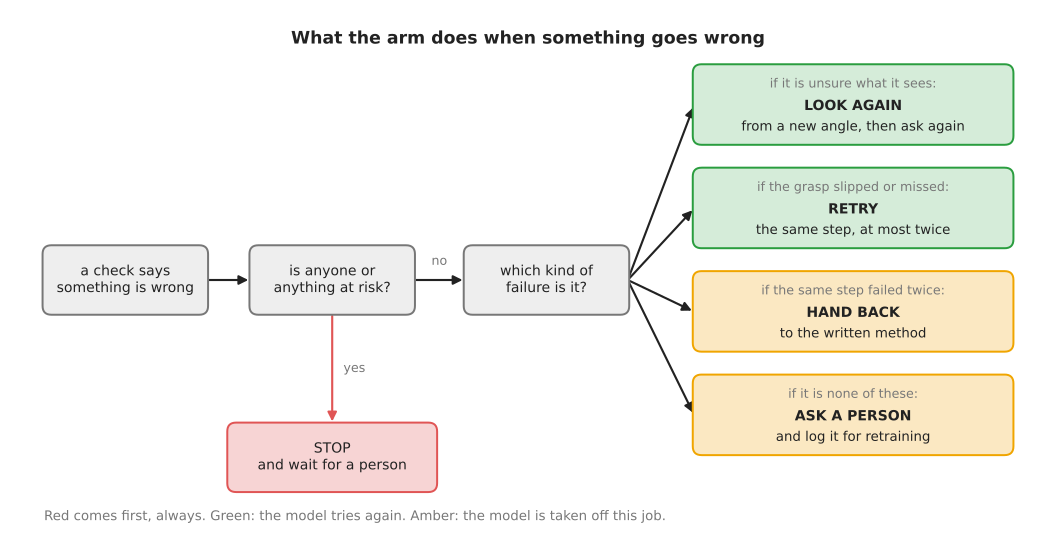
First something must notice the failure, and that can be either a programmed check, such as "the gripper closed fully, so it holds nothing", or a learned failure detector. Once the failure has been noticed, the arm chooses one of five responses, and the order below matters.
- Stop. If anything or anyone is at risk, the arm stops and waits for a person. This comes before everything else, and it is done by the safety monitoring layer, not by the model.
- Look again. If the model was unsure what it saw, the arm moves the camera to a new angle and asks the model again. The uncertainty and confidence page shows how to tell when a model is unsure.
- Retry. If a grasp slipped or missed, the arm tries the same step again. It keeps a count, and it gives up after a set number, often two. Without a count, an arm can retry the same failing grasp for ever.
- Hand back to the written method. If the model fails the same step twice, the arm switches to a programmed method for this one job, if there is one. For example, a slow and careful top-down grasp worked out from the geometry of the mug. Such a method is less clever than the model, however it behaves the same way every time, which is exactly what you want after two failures. Book 3's programmed methods page describes such methods.
- Ask a person. If none of these apply, the arm stops the job and asks for help. The trial is saved, so it can become a new training example.
Every one of these five responses should also be logged, exactly as section 5 describes, because a model that succeeds only after two retries is not as good as its success rate alone would suggest.
8. From simulation to the real arm#
Running enough real trials takes a long time, which is why people try to do some of the work elsewhere first. A simulator, meaning a program that pretends to be the real world, can run thousands of trials overnight, so a common plan is to test in simulation first and to run real trials only for the models that pass. The difference between how a model does in simulation and how it does on the real arm is called the sim-to-real gap.
Three methods shrink that gap. Other pages explain each of them in full, so this section only says how they fit into evaluation.
- Domain randomisation. The simulator changes colours, light, masses and friction at random during training, so the real world looks like one more random variation. Where the data comes from explains it.
- System identification. You measure your real arm, such as its delays and frictions, and set the simulator to match. Book 6's system identification page shows how.
- Test in simulation first. Use the simulator as a filter, because a model that fails in simulation will almost certainly fail on the arm as well. A model that passes has earned real trials, and nothing more than that.
Book 3's sim-to-real section separates the gap into three parts: how things look, how the arm moves, and how things feel when touched. It explains that the first two now have good answers and the third does not, so for any job where the grip matters a simulated success rate tells you very little. Keep the two numbers apart by reporting the simulated rate and the real rate separately, and never let a simulated rate stand in for a real one.
9. A worked example: a mug-picking model, from test set to 100 trials#
The sections above cover each part of evaluation separately, so here is the whole process for one job, from beginning to end. A movement model has been fine-tuned to pick a mug from a rack and put it on a tray, and the old way of doing the job is a written method that works out a grasp from the mug's shape.
- Test set. On kept-back demonstration steps the model's actions are very close to the person's, which shows that the training worked. However it does not show that the arm will succeed, for the three reasons given in section 2.
- Simulation. In a simulated copy of the rack the model succeeds in most trials, which is enough to justify trying it on the real arm, slowly, with a person at the emergency stop.
- Twenty real trials. The model succeeds 18 times, while the written method succeeds 15 times on the same 20 setups. The two ranges are 68.3% to 98.8% and 50.9% to 91.3%, so they overlap far too much to say the model is better.
- A hundred real trials each. On a fixed list of 100 setups, in mixed order, the model succeeds 90 times and the written method 75 times. The ranges are 82.4% to 95.1% and 65.3% to 83.1%. They only just overlap. The model is probably better, and a paired comparison on the same setups would say how sure that is.
- Sort the failures. The model's 10 failures sort as in the picture in section 6: 5 slips while lifting, 2 reaches for the wrong spot, 1 timeout, 1 safety stop on the rack and 1 time a person stepped in.
- Fix the largest kind. The slips all happened with the heaviest mug. The team adds demonstrations of lifting heavy mugs and fine-tunes again.
- Run the same 100 setups again. This gives a new count and a new sorted list, which can be compared with the old one setup by setup.
- Set the failure plan. For the job on the real line, a slip leads to one retry, and a second slip hands the job to the written method.
The test set says the training worked, the simulation says the model is worth trying, and only the real count, with its range, says how good it is.
10. Where it is used on a robot arm#
The ideas on this page apply to every learned model on an arm, not only to movement models.
- Movement policies. Success rate over real trials is the standard measure for behaviour cloning, action chunking and vision-language-action models.
- Grasp models. Grasp success is counted over real pick attempts, usually on a fixed set of objects. See the grasp models chapter.
- Seeing models. A detector's test-set score is only the start. What counts is how often the arm reaches for the right object.
- Automatic judging. Counting successes by hand is slow. A reward and progress model can judge success from video, but it is a model too, and it must be checked against a person on some trials.
- Monitoring after deployment. Once the arm is working, the same log keeps running. A success rate that slowly falls means something has changed: the lighting, the objects, or a camera that has moved.
11. What goes wrong, and what people do about it#
The table below lists the common mistakes in evaluation. Read each row across: the mistake, the sign you would see, and what people do instead.
| Mistake | The sign you would see | What people do instead |
|---|---|---|
| trusting the test set score | a near-perfect score, then poor real trials | run real trials; treat the test set as a check that training worked |
| too few trials | a model that "won" last week loses this week | report the confidence interval; run about 100 trials for a decision |
| the same easy setups every time | high success rate, then failures on the real line | a fixed list that covers the real range of positions, objects and light |
| success judged loosely afterwards | near misses counted as wins | write the success rule down before the first trial |
| only the failures logged | no way to see how close the successes came to failing | log every trial the same way |
| failures not sorted | effort spent on rare failures | sort and count, and fix the largest kind first |
| simulated and real rates mixed | a quoted rate that the arm never reaches | report them separately |
| no plan for failure | the arm retries for ever, or carries on with nothing in the gripper | a written failure plan with a retry count and a stop |
12. Libraries and tools#
The table below lists real tools for each part of evaluation. Read each row as one tool: what it is for, and a note on when to use it.
| Tool | What it does | Note |
|---|---|---|
lerobot-eval (LeRobot) | runs a trained LeRobot policy on simulated benchmarks through one shared harness, and reports the success rate | for testing in simulation first; Book 3's section 9 describes it |
| LeRobot's recording tool, given a policy | runs a trained policy on a real arm and saves each run as an episode, with pictures and actions | gives you the per-trial log of section 5 for LeRobot arms |
| SciPy | scipy.stats.binomtest(k, n).proportion_ci(method='exact') gives the Clopper-Pearson interval | one line for any count of successes |
| statsmodels | statsmodels.stats.proportion.proportion_confint(k, n, method='beta') gives the same interval | handy if you already use statsmodels |
| ROS 2 bags | ros2 bag record saves every message on the robot, such as pictures, joint states and commands | for arms run with ROS |
| Rerun, Foxglove | viewers that replay logged pictures, joint positions and actions on one timeline | the fastest way to see why a trial failed |
| a spreadsheet | one row per trial: setup, result, failure kind, note | the simplest way to sort and count failures |
13. Why this rather than the obvious alternative, and what it costs#
This section answers the four questions for evaluating a model on an arm: what it is, what it does for you, why it rather than the obvious alternative, and what it costs.
It is a way of deciding whether a model is ready: real trials on fair setups, counted with a confidence interval, every trial logged, every failure sorted, and a written plan for what the arm does when it fails. It gives you a number you can trust and a list of what to fix next.
The obvious alternative is to trust the test set score, or to run a handful of trials and see whether it "looks good". Both are cheap. Both are misleading. The test set score measures single steps against a person's answer, not whole trials, as section 2 showed. A handful of trials gives a range so wide, 55.5% to 99.7% for 9 of 10, that it cannot tell a poor model from a good one. And neither says anything about what the arm does when the model is wrong, which is what decides whether it is safe to use.
The costs are real:
- Time. A hundred real trials of a 30-second job, with resetting the scene, is most of a day. Comparing two models is two days.
- Storage. Logging pictures from every trial fills disks quickly.
- Care. Fair setups, a written success rule and mixed order take discipline.
- Repetition. Every change to the model, the gripper or the room means running the trials again.
The time is worth it before a model runs unattended. For early experiments, 20 trials are enough to spot a model that is clearly broken, as long as you remember how wide the range is.
14. Where to read next#
- Uncertainty and confidence shows how to tell when a model is unsure, which decides when the arm should look again or ask.
- Running a model on a robot describes the loop and the safety checks around a model.
- Fine-tuning shows how to train on the failures you sorted.
- Book 3's simulation and evaluation covers simulators, sim-to-real and the public benchmarks, and why their numbers are hard to compare.
- Collision and failure detection covers the models that notice a failure while it happens.
- Book 6's safety monitoring covers the programmed checks that stop an arm whatever the model says.
15. Using it in Python#
Sections 3 and 6 are the two parts of evaluation that need a computer at all, since the trials themselves are run by hand. This section shows both, because together they are about ten lines, and after reading it you will be able to turn a list of trials into the confidence interval and the sorted failure counts that the rest of this page argues for.
import collections

from scipy.stats import binomtest

# One entry per trial, written down as section 5 says, while the trials are running.
trials = [{'setup': 1, 'success': True, 'failure_kind': None},
          {'setup': 2, 'success': False, 'failure_kind': 'slip while lifting'},
          # ... one more line like these for every trial you ran
          ]

successes = sum(t['success'] for t in trials)
interval = binomtest(successes, len(trials)).proportion_ci(method='exact')
print(f'{successes} of {len(trials)} = {successes / len(trials):.0%}, '
      f'95% interval {interval.low:.1%} to {interval.high:.1%}')

kinds = collections.Counter(t['failure_kind'] for t in trials if not t['success'])
for kind, count in kinds.most_common():
    print(f'{count:3d}  {kind}')
With 90 successes in 100 trials the first line prints 90 of 100 = 90%, 95% interval 82.4% to 95.1%, which is the row in section 3's table, so this really is the whole
calculation.
SciPy gives you the hard part in one call. binomtest(k, n) describes the count, and
its proportion_ci(method='exact') returns the Clopper-Pearson interval of section 3,
so you never see the formula. Python's own collections.Counter does the sorting of
section 6, and most_common() returns the kinds in order, largest first, which is the
order in which you should fix them. Neither needs anything installed beyond SciPy.
What you have to collect yourself is trials, and that is the work. Every entry costs a
real attempt on the real arm, with the scene reset in between, so a hundred trials of a
thirty-second job is most of a day, as section 13 says. You also have to write the
success rule down before the first trial and keep the list of failure kinds short
enough that each failure clearly belongs to exactly one of them, because a kind that
overlaps another gives counts nobody can act on.
What you have to decide is the number of trials and the list of kinds. Section 3 gives
the arithmetic for the first: about a hundred trials for a decision, and twenty only to
spot a model that is obviously broken. If you already use statsmodels, then
statsmodels.stats.proportion.proportion_confint(k, n, method='beta') gives exactly the
same interval, and for trials in a simulator rather than on the arm, LeRobot's
lerobot-eval runs them and reports the success rate for you.