A neuron multiplies each of its inputs by a weight, adds those results together and adds a bias. One neuron worked all of that out by hand, and the two pages since have used the result without questioning it. All three ended on the same limit: whatever values a neuron's weights and bias take, the line that divides its yes from its no stays straight. This page is about the one small rule that removes that limit. The rule is applied to the weighted sum before the neuron hands its answer on, and it is called an activation function. The number that comes out of it is the neuron's activation, which is where the rule gets its name.
This page says in several places what a rule does to training, even though training is explained only in the next chapter, because the choice between one rule and another is mostly a choice about how well training goes.
When you reach the end of this page you will know why a network built only from multiplying and adding collapses into a single straight line however many layers it has, what the rule at the end of each neuron adds, why the models built today mostly use a smoothed version of the simplest rule rather than the simplest rule itself, and why the rule after the very last layer is not a choice at all but is decided by the kind of answer the job needs.
Contents#
- Why multiplying and adding is not enough
- What any rule has to have
- The rectified linear unit
- GELU and SiLU, and why networks use them now
- The rule at the end of the network
- Where to read next
- Using it in Python
1. Why multiplying and adding is not enough#
The page before this one ended on a limit. Whatever values a neuron's four numbers take, the line between yes and no stays straight. Many jobs on a robot need an answer that rises and then falls, and a straight line cannot give one. This section is here because that limit is the reason a neuron has a rule at the end. You saw the rule in what one neuron is made of, and you saw the fitted line of what a model is work without one. This section shows what the rule is for with worked numbers. What any rule has to have then says which rules can do the job, and the rectified linear unit describes the simplest of them. The answer comes in three steps. First, many jobs need an output that bends, and one neuron without the rule can only draw a straight line. Second, putting more neurons in a row does not fix this if nothing comes between them. Third, the rule between them does fix it.
Start with a job that a straight line cannot do. The brightness of the patch is one of those jobs. A patch that is nearly black shows nothing, and a patch that is completely white shows nothing either. So brightness is good in the middle and bad at both ends.
The picture below draws what we want from the brightness, which is a shape that rises to the middle and falls again, and it draws the best straight line through that shape.
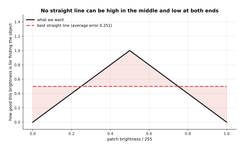
The best straight line through this target is flat at 0.499, and it is wrong by 0.251 on average. A straight line cannot be high in the middle and low at both ends, so no choice of weight and bias fixes this.
The obvious fix is to use more than one neuron, one after the other. The rest of this section shows that this fix does nothing on its own. Multiplying by a weight and adding a bias can only ever make a straight line, and two of these neurons in a row are exactly equal to one neuron with different numbers.
The picture below puts one reading through two neurons, one after the other, with nothing applied between them.
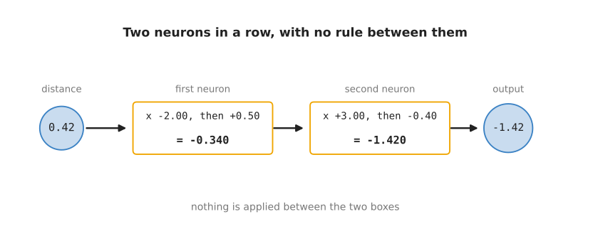
The first neuron turns 0.42 into -0.340. The second neuron turns -0.340 into -1.420.
The picture below puts the same reading through a single neuron instead, and that neuron gives the same answer.
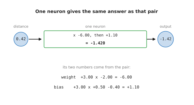
One neuron with the weight -6.00 and the bias +1.10 turns 0.42 straight into -1.420, without the stop in the middle.
The reason is ordinary arithmetic. The second neuron multiplies what it receives by 3.00, and what it receives is -2.00 times the distance plus 0.50. So the pair works out 3.00 times -2.00 times the distance, which is -6.00 times the distance. It also works out 3.00 times 0.50 and then subtracts 0.40, which gives 1.10. In other words the two weights multiply together, and the first bias is scaled by the second weight.
The picture below draws both of those roads across the whole sweep of distances, and it adds a third line in which the rule is applied between the two neurons.
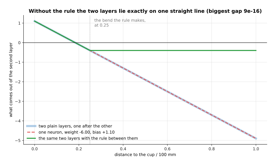
Across the whole sweep the two plain layers and the single neuron never differ by more than 0.0000000000000009, which is as close as the computer can measure. The third line, which has the rule between the two neurons, bends at a distance of 0.250 and is a different shape altogether.
The same collapse happens however many neurons you chain together. This is worth checking, because it is easy to believe that three in a row must be able to do something that two cannot.
The picture below is a table with one row for each of three layers in a row, and one last row for the single neuron that replaces all three. Read each row from left to right, and compare the two numbers in the last column.
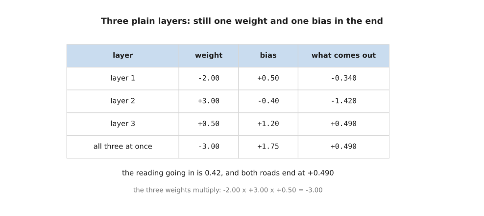
The three weights multiply to -3.00, and the three biases gather into +1.75. So three layers in a row give exactly the same +0.490 that one layer with those two numbers gives.
So a network made only of multiplying and adding could have a thousand layers and would still only be able to draw one straight line. That brings back the brightness job from the start of this section.
The picture below does the same job with two neurons that each apply the rule, and it draws what each of those neurons gives as well as their total.
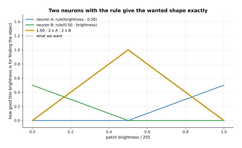
Two neurons with the rule rebuild the wanted shape exactly, and the biggest gap anywhere between the two lines is zero.
That is what the rule at the end of each neuron is for. Without it, any number of neurons collapses into one straight line. With it, a few neurons can bend the line into the shape a job needs. Everything in this section used particular numbers and one particular rule, so what any rule has to have does the same working with letters, to find out which rules would do the same job.
2. What any rule has to have#
The section before showed the collapse and its cure with particular numbers. This section does the same working with letters in place of the numbers, so that it holds for every weight and every bias. From that it says which properties a rule needs, and which it does not.
Write a neuron with one input as a weight times the input, plus a bias. Call the first neuron's weight and bias w1 and b1, and the second neuron's w2 and b2. The first neuron reads the distance d, and the second reads what the first gives. The lines below follow the arithmetic through, one step per line.
first neuron:    s = w1 x d + b1
second neuron:   y = w2 x s + b2
put s in:        y = w2 x (w1 x d + b1) + b2
multiply out:    y = (w2 x w1) x d + (w2 x b1 + b2)
The last line has the shape of one neuron. Its weight is w2 x w1, and its bias is w2 x b1 + b2. No step in that working depended on which numbers the letters stand for. Putting in w1 = -2.00, b1 = +0.50, w2 = 3.00 and b2 = -0.40 gives the weight -6.00 and the bias +1.10 from the section before. A neuron with several inputs works the same way, with one weight for each input. So does a chain of three neurons, or a thousand, because each step takes a straight line and gives back a straight line.
Now put a rule between the two neurons, and call it f. The second neuron then gives y = w2 x f(w1 x d + b1) + b2. Whether the pair still collapses into one neuron depends only on f.
Suppose f is itself a straight line, such as f(s) = 0.5 x s + 0.2. Then f is one more multiply and one more add, and the working above absorbs it. The pair becomes one neuron with the weight w2 x 0.5 x w1 and the bias w2 x (0.5 x b1 + 0.2) + b2. The picture below draws that with the same two neurons as before.
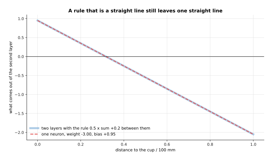
The two layers with the straight rule between them lie exactly on the line of one neuron with the weight -3.00 and the bias +0.95. At a distance of 0.42 both give -0.310. So a rule that is a straight line changes nothing, whatever its two numbers are.
That gives the first property, and it is the one that matters most. The rule must not be a straight line. A rule like that is called nonlinear. One corner is enough. The rectified linear unit is two straight pieces joined at 0, and that corner stops the working above, because f(w1 x d + b1) can no longer be written as one multiply and one add.
Being nonlinear is very nearly enough. In 1993, Moshe Leshno, Vladimir Lin, Allan Pinkus and Shimon Schocken proved that one layer of neurons, added up at the end, can follow any shape without breaks over a limited range of readings, as closely as you ask. It needs enough neurons, and a rule that is not a polynomial. A polynomial is a rule built only from powers of the sum, such as s x s. A rule like that keeps the whole network a polynomial with a fixed highest power, and that limits its shapes however many neurons it has. The proof also asks that the rule never runs off to infinity at any one sum, and every rule on this page meets that. The six and twelve elbows in the rectified linear unit are a small case of this result.
That result says good weights exist. It says nothing about how to find them. The training methods in the next chapter find them by moving each weight a little in the direction that improves the answer. They learn that direction from the slope of the rule, which is how much the output moves when the sum moves a little. So the second property is that the rule has a slope that is not 0 over a useful part of its range.
The step rule shows why this is a separate property. It gives 0 for any sum at or below 0, and 1 for any sum above. The picture below draws it.
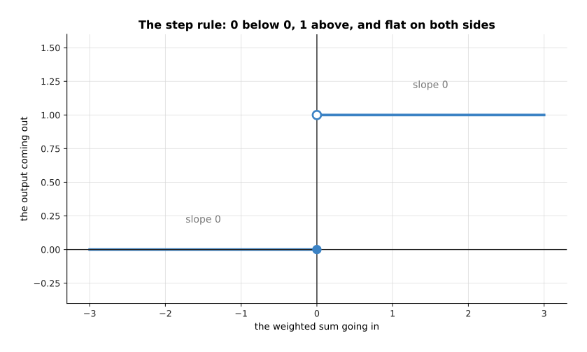
The step rule is not a straight line, so it has the first property. But it is flat on both sides of the jump, so its slope is 0 everywhere except at the jump, where it has no slope at all. Moving a weight a little changes nothing that the step gives, so training gets no direction. The earliest artificial neurons, in the 1950s, used this rule. Networks with several layers moved to rules with a slope in the 1980s, once training by slopes arrived, for exactly this reason.
A third property is worth having but is not required. The rule should be cheap to work out, because it runs once for every neuron. GELU and SiLU shows that this matters less than it seems.
Some properties look necessary and are not. The rule does not have to stay inside a range, because the rectified linear unit grows without limit. It does not have to be smooth, because the rectified linear unit has a corner. It does not have to rise all the way, because GELU and SiLU dip below 0 and come back up. Those differences decide how well training goes, not whether a network can bend.
So every rule in use is nonlinear and has a slope over most of its range. The rules differ in where they bend and what slope they give. The rectified linear unit looks at the simplest rule with both properties, and at the places where its slope gives out.
3. The rectified linear unit#
The section before said that a rule needs a bend and a slope. This section looks at the simplest rule that has both. It is called the activation function, which means a rule that is applied to the weighted sum to give the neuron's output. The number that comes out of it is called the neuron's activation. The simplest one, and the one networks have used the longest, is the rectified linear unit, which is usually shortened to ReLU. The whole of it is this: if the sum is below 0 give 0, and otherwise give the sum unchanged.
The picture below draws that rule on ordinary axes. The number going in is on the bottom axis, and the number coming out is on the side axis.
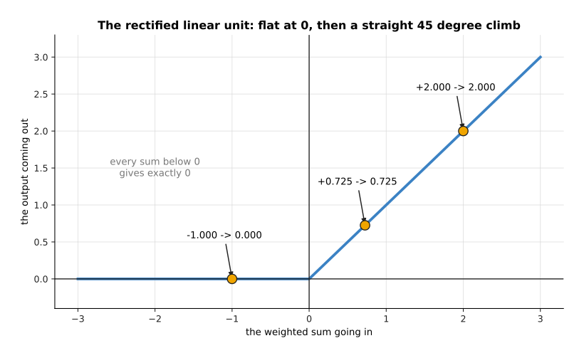
The table below gives the output of the rule for eight different sums. Read one row at a time: the left column is the number going in, and the right column is the number coming out.
| weighted sum going in | output of the rule |
|---|---|
| -2.000 | 0.000 |
| -1.000 | 0.000 |
| -0.500 | 0.000 |
| 0.000 | 0.000 |
| +0.500 | 0.500 |
| +0.725 | 0.725 |
| +1.000 | 1.000 |
| +2.000 | 2.000 |
Every number below 0 becomes 0, and every number above 0 is passed on untouched. Our own neuron had a sum of +0.725, which is the sixth row, so its output is 0.725 as well.
This rule looks too simple to do any work. The reason it does so much work is the corner at 0. A neuron with this rule is two different things joined at one point, because on one side of the corner it ignores its inputs and on the other side it follows them exactly. The place where it changes is the point that what changes when a weight or the bias changes moved with the bias, and this page calls that point the elbow. Once several neurons each have an elbow in a different place, the elbows can be added together into any shape at all.
The picture below shows that. It draws a smooth curve, and then it draws two lines made of straight pieces that follow the curve, one with six elbows and one with twelve.
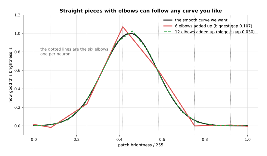
Six neurons with elbows at 0.08, 0.25, 0.42, 0.58, 0.75 and 0.92 follow the smooth curve to within 0.107 everywhere. Twelve of them bring that largest gap down to 0.030.
That is the answer to the question that why multiplying and adding is not enough raised. A network can bend because each neuron can switch itself off, and a network with more neurons can bend in more places. What this costs is that half of every neuron's range gives nothing at all.
The picture below shows the cost directly. It takes our own neuron, sweeps both the distance and the gripper opening, and colours the output after the rule.
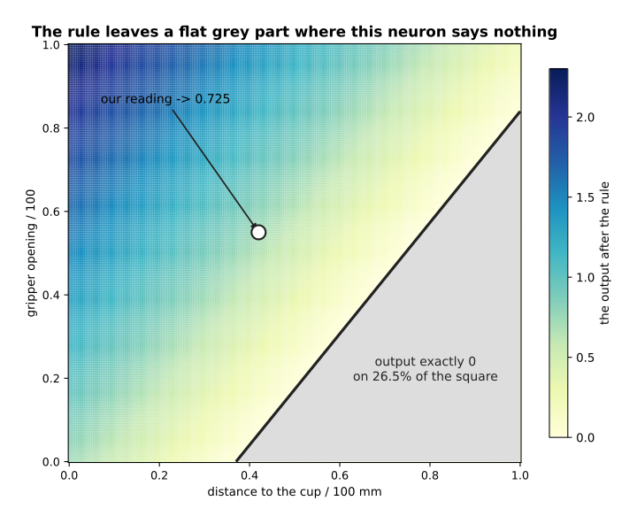
The grey part of that square is where the output is exactly 0, and it covers 26.5 per cent of the square. Inside the grey part the neuron says the same thing about every pair of readings, so it says nothing useful about them at all.
A neuron is worse off still if its sum is below 0 for every reading it ever meets, because then it gives 0 all of the time.
The picture below simulates 64 neurons with randomly chosen weights, gives each of them the same 200 simulated moments to read, and draws one square for each neuron. The number in a square is the percentage of the 200 moments on which that neuron gave something above 0.
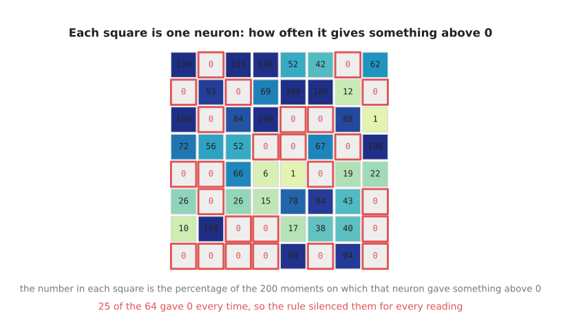
Of those 64 neurons, 25 never gave anything above 0, and the average neuron answered on 36.6 per cent of the moments. The readings and the weights here are simulated, and they are drawn from a fixed starting point so that the picture can be made again.
A neuron in that state is called a dead unit, and it is dead in a strong sense. The training methods in the next chapter move each weight a little in the direction that would improve the answer. A neuron whose output is 0 for every example gives no direction to move in. The reason shows up in the slope of the rule, where the slope means how much the output moves when the number going in moves a little.
The picture below draws that slope. The number going into the rule is on the bottom axis, and the slope of the rule at that number is on the side axis.
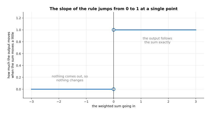
To the left of 0 the slope is 0, which means that moving the sum a little changes nothing at all. To the right of 0 the slope is 1, which means the output follows the sum exactly. At the point 0 itself there is no single slope, because the rule jumps from one value to the other.
That flat left half and that jump at 0 are the two weak points of this rule. The next section, GELU and SiLU, describes the newer rules that fix both, and those are the rules you will find inside most models built today.
4. GELU and SiLU, and why networks use them now#
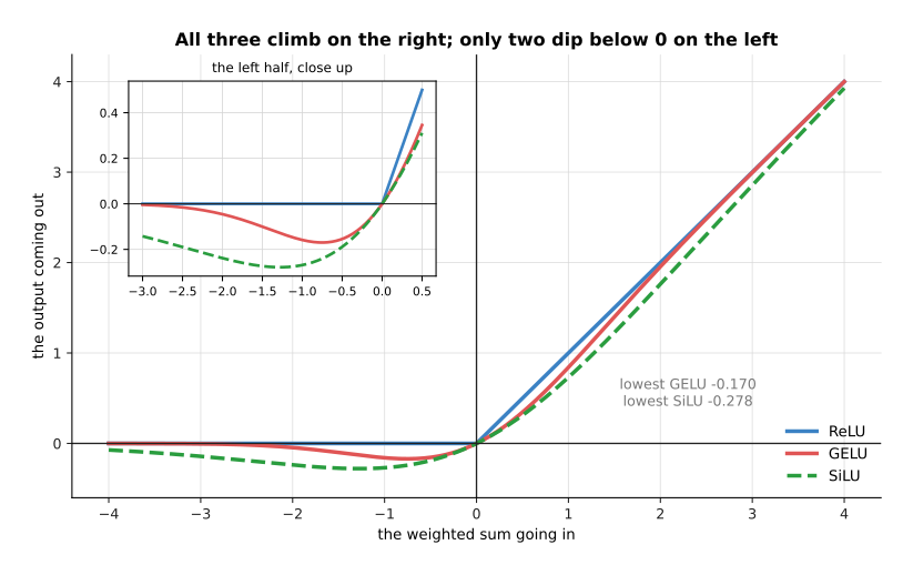
The section before ended on two weak points of the rectified linear unit: a flat half where training gets no direction, and a jump at 0. This section is here because the models you will meet later in this book mostly use a rule that fixes those two points. Two smoother rules have taken over much of the rectified linear unit's work in the models built today. Both of them keep its shape and round off its corner. They are the Gaussian error linear unit, shortened to GELU, and the sigmoid linear unit, shortened to SiLU and also called swish. The rectified linear unit switches flatly between 0 and 1: it multiplies the sum either by 0 or by 1 and by nothing in between. GELU and SiLU instead multiply the sum by a number between 0 and 1 that grows as the sum grows.
The picture below draws all three rules on the same axes, and the small box inside it repeats the left half of the same picture at a larger size.
The table below gives what each rule produces for the same eight sums that the rectified linear unit used. Read one row at a time: the first column is the sum going in, and the other three columns are what each rule gives for that sum.
| sum going in | ReLU | GELU | SiLU |
|---|---|---|---|
| -2.000 | 0.0000 | -0.0455 | -0.2384 |
| -1.000 | 0.0000 | -0.1587 | -0.2689 |
| -0.500 | 0.0000 | -0.1543 | -0.1888 |
| 0.000 | 0.0000 | 0.0000 | 0.0000 |
| +0.500 | 0.5000 | 0.3457 | 0.3112 |
| +0.725 | 0.7250 | 0.5552 | 0.4884 |
| +1.000 | 1.0000 | 0.8413 | 0.7311 |
| +2.000 | 2.0000 | 1.9545 | 1.7616 |
All three rules give almost the same answer for a large sum. At +2.000 the rectified linear unit gives 2.0000, GELU gives 1.9545 and SiLU gives 1.7616. On the left they differ more. At -1.000 the rectified linear unit gives 0.0000, while GELU gives -0.1587 and SiLU gives -0.2689. The lowest number GELU ever gives is -0.170, and the lowest SiLU ever gives is -0.278.
That small dip below 0 is the first difference. It means that a neuron whose sum is a little below 0 still gives a small answer rather than nothing, so such a neuron is never completely dead. The second difference is in the slope, and the slope is what the training methods in the next chapter actually use.
The picture below draws the slope of each of the three rules on the same axes.
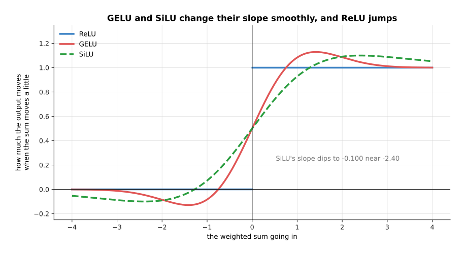
The rectified linear unit's slope is 0 at an input of -2 and 1 at +2, with a jump between them. GELU's slope runs from -0.0852 at -2 to +1.0852 at +2, and SiLU's runs from -0.0908 to +1.0908. Both of the smooth rules dip below 0 on the left, GELU down to -0.129 near -1.42 and SiLU down to -0.100 near -2.40.
The picture below puts the three rules back on the neuron from what one neuron is made of. The left half sweeps the scaled distance from 0 to 1, which is 0 to 100 millimetres, and the right half is the same sweep again with the area around the elbow made larger.
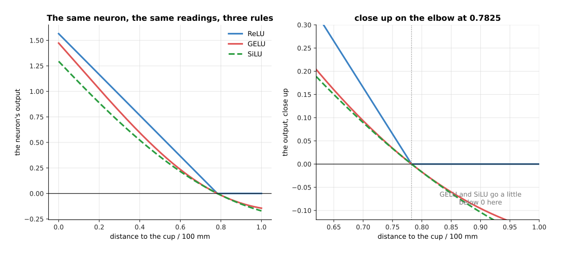
At our reading of 0.42 the sum of +0.725 becomes 0.7250 under the rectified linear unit, 0.5552 under GELU and 0.4884 under SiLU. At a distance of 0.85, where the sum is -0.1350, the rectified linear unit gives exactly 0, while GELU gives -0.0603 and SiLU gives -0.0630.
The dead units of the rectified linear unit are the clearest case where that difference matters. The picture below takes the same 64 simulated neurons and the same 200 simulated moments, replaces the rule with GELU, and writes in each square the average size of the slope that neuron gets. The 25 neurons that the rectified linear unit had silenced are outlined in red.
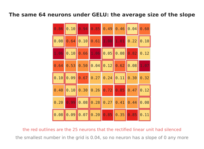
Under the rectified linear unit those 25 neurons have a slope of exactly 0 on all 200 moments, so training cannot move them. Under GELU the same 25 neurons have an average slope size between 0.0400 and 0.3466. The smallest number anywhere in the grid is 0.0400, so no neuron is left with a slope of 0.
So why use the smooth rules rather than the rectified linear unit, which is simpler and older? The first reason is the one the pictures above show, which is that the slope changes smoothly and gives the training methods something to work with everywhere, instead of nothing on one side and a jump in the middle. The second reason is that the large models built today train a little more steadily with them. Most transformer models, which the chapter the transformer explains, use GELU or SiLU inside. The rectified linear unit stays common in smaller vision models and wherever speed matters most.
What the smooth rules cost is arithmetic. The rectified linear unit is a single comparison against 0. GELU and SiLU both need a curve that a computer works out from a longer calculation, and that calculation takes several times as long for each number. That extra cost looks large until you count how often each of the two things happens inside one layer.
The picture below counts both things for one layer that takes 1,024 numbers in and has 1,024 neurons. The left bar is the multiply-adds, where one multiply-add means one weight multiplied by one number and added to a running total. The right bar is the number of times the rule is used. The side axis grows by a factor of ten at each step, because one bar is a thousand times the other.
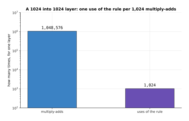
That layer does 1,048,576 multiply-adds and uses the rule only 1,024 times, which is one use of the rule for every 1,024 multiply-adds.
The picture below turns that ratio into the extra work for the whole layer. Each bar assumes that one use of the rule costs as much as a given number of multiply-adds, and it gives the extra work as a percentage.
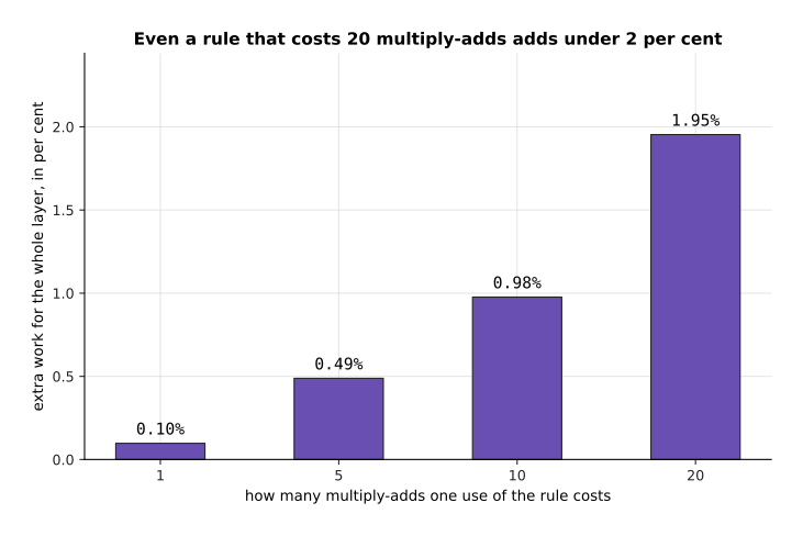
Even a rule that costs as much as 20 multiply-adds adds only 1.95 per cent to the work of that layer. So the dearer rule is worth its price whenever it trains better.
Those two pictures also introduce the subject of layers, depth and width, which is that a layer of 1,024 neurons holds over a million weights, and that those weights are arranged in a grid which a computer multiplies in one go.
Everything so far has been about the rule inside a network, where you are free to choose. The rule at the end of the network deals with the last layer, where you are not.
5. The rule at the end of the network#
The four sections before this one were all about the rule that follows a hidden layer, and for those layers the rule is a free choice: you weigh the rectified linear unit against GELU and SiLU and pick one. This section is here because the last layer is not like that. The rule after the output layer is decided by the job, not by you, and picking it wrongly produces answers that cannot mean what they are supposed to mean.
The reason is simple. A rule is the last thing that touches a number before anybody reads it, so the rule decides which answers are even possible. The rectified linear unit can give 7.3. If the answer is supposed to be a probability, 7.3 is not a wrong probability; it is not a probability at all. So the question to ask is what the answer has to look like, and the rule follows from that.
The table below gives the four cases you will meet. Read it a row at a time: the first column is what the job needs, the second is the rule that produces it, and the third says why that rule and not another.
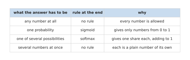
The first row is the easiest and the one people forget. If the answer is a plain measurement, such as how many millimetres the tool tip has dropped, then no rule belongs at the end at all. Any number is a valid answer, so squeezing the output into a range would only throw away answers that were correct.
The second row is the one this chapter has been quietly using. When the answer is one probability, the rule is the sigmoid, which takes any number at all and gives back a number between 0 and 1. The smallest network and a network on a robot both ended on it without explaining it, and this is that explanation.
The picture below draws the sigmoid, with the totals of the three moments of the grasp example marked on it.
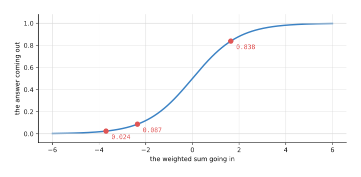
A sum of 0 comes out as exactly 0.500, meaning the network is saying it has no idea. The total of +1.645 when the gripper is ready to close comes out as 0.838. The total of -2.355 when it is aimed beside the cup comes out as 0.087, and the total of -3.700 when it is too far away comes out as 0.024. The curve never reaches 0 or 1, however large the sum gets: at -6 it gives 0.0025 and at +6 it gives 0.9975.
That last fact has a consequence worth knowing. The curve is nearly flat at both ends, so once a sum is past about 6 in either direction, making it larger changes the answer hardly at all. The interesting part of the sigmoid is the middle, and a network whose sums all land far out at the ends has stopped saying anything useful. The same flatness is what the rectified linear unit ran into on its left half, and for the same reason: a flat rule gives training nothing to work with.
The third row covers an answer that picks one of several named possibilities, such as which of three tools to fit. The output layer then has one neuron for each possibility, and the rule is softmax, which turns their totals into shares that add up to 1. With totals of +0.40, +2.10 and -0.70 the three shares come out as 0.147, 0.804 and 0.049, which add to exactly 1.000. Reading them as probabilities is only honest because they add up, and that is the whole reason softmax exists rather than using a sigmoid on each neuron separately.
The fourth row is the case where the answer is several ordinary numbers at once, such as three coordinates for where to put the gripper. Those are measurements, not shares, so nothing should tie them together and no rule belongs at the end.
So the habit worth building is to settle the shape of the answer first. That fixes how many neurons the output layer has and which rule follows it, and only then is anything in the middle worth thinking about.
6. Where to read next#
- Layers, depth and width is the next page. It joins many neurons, each with the rule from this page at its end, into a layer, and then stacks the layers.
- What a network can learn takes the elbows of the rectified linear unit and shows that enough of them will follow any shape at all.
- Backpropagation explains why the slopes drawn in the rectified linear unit and GELU and SiLU matter so much, because those slopes are what training reads.
- Normalisation and stability deals with the other half of keeping a deep network trainable, which is holding the numbers that reach each rule in a sensible range.
- A transformer block is where you meet GELU and SiLU again, inside the models most of this book is about.
7. Using it in Python#
The three rules are one function call each in PyTorch, which is the library most of this book's models are built with. The code below takes the same weighted sum of +0.7250 that one neuron worked out, and the sum of -0.1350 that the same neuron gives at a distance of 0.85, and puts both through all three rules.
import torch

above = torch.tensor([0.7250])                                 # the sum at 0.42
print(f"{torch.relu(above).item():.4f}")                       # 0.7250
print(f"{torch.nn.functional.gelu(above).item():.4f}")         # 0.5552
print(f"{torch.nn.functional.silu(above).item():.4f}")         # 0.4884

below = torch.tensor([-0.1350])                                # the sum at 0.85
print(f"{torch.relu(below).item():.4f}")                       # 0.0000
print(f"{torch.nn.functional.gelu(below).item():.4f}")         # -0.0603
print(f"{torch.nn.functional.silu(below).item():.4f}")         # -0.0630
The first three numbers are the three rules disagreeing mildly about a sum that is above 0, and the last three are the same rules disagreeing about a sum that is below it. The rectified linear unit throws the negative sum away completely, while the two smooth rules keep a small part of it, and that small part is the whole difference that GELU and SiLU is about.
In a real model you rarely call these functions by name on their own. You put one
after each layer, and the library applies it to every number the layer produced.
The output rules work the same way: torch.sigmoid and
torch.nn.functional.softmax are the two from
the rule at the end of the network.
Layers, depth and width shows that arrangement, and
using it in Python on that page
builds a stack of layers with a rule between each pair.